8.1. HOW THE IMF AFFECTS STELLAR DEMOGRAPHY

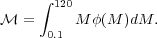
For a fixed amount of gas turned into stars, different IMFs obviously imply different proportions of low mass and high mass stars. This is illustrated in Figure 8.1 showing three different IMFs, all with the same slope below 0.5 M, that is s = 1 + x = 1.35, and three different slopes above:

(1)

where the factor 0.5^1.3-s ensures the continuity of the IMF at M = 0.5 M. The normalization of the three IMFs corresponds to a fixed amount of gas turned into stars, that is, for fixed

(2)

Here the case s = 2.35 corresponds to the Salpeter-diet IMF already encountered in previous chapters. Thick lines in Figure 8.1b show the cumulative distributions, defined as the number of stars with mass less than M, N(M' < M) = ∫_0.1^M (M') dM', while thin lines show the fraction of mass in stars less massive than M. In a Salpeter-diet IMF ~ 0.6% of all stars are more massive than 8 M, while for s = 3.35 and 1.5 these fractions are 0.03% and 9 % respectively. The mass in stars heavier than 8 M is 20% for a Salpeter-diet IMF; it drops to 1% for s = 3.35, and is boosted to 77 % for s = 1.5, a top-heavy IMF. Figure 8.1 wants to convey the message that IMF variations have a drastic effect on stellar demography, and therefore on several key properties of stellar populations. Suffice it to say that most of the nucleosynthesis comes from M > 10 M stars, whereas the light of an old population (say, t > 10 Gyr) comes from stars with M 1 M, and therefore is proportional to (M = M).

Figure 8.1. Left: three different IMFs normalized to have the same total stellar mass of 1 M. Below 0.5 M all three IMFs have the same slope s = 1.3 and above it s = 1.5, 2.35 (Salpeter) and 3.35, shown as dashed, solid, and dot-dashed lines, respectively. Right: cumulative distributions of the number (thick lines) and of the stellar mass (thin lines) for the three IMFs with the same line encoding as in the left panel.

Figure 8.2 shows the variation of scale factor A (cf. Chapter 2) as a function of the IMF slope, again for a fixed amount of gas turned into stars. The scale factor A has a maximum for s 2.75, pretty close to the Salpeter's slope. Since by construction A = (M = 1 M) and the luminosity of a > ~ 10 Gyr old population is proportional to (M = 1 M), an IMF with the Salpeter's slope has the remarkable property of almost maximizing the light output of an old population, for fixed mass turned into stars. A flat IMF (s = 1.35) is much less efficient in this respect, indeed by a factor of ~ 8 compared to the Salpeter's slope, as shown by Figure 8.2. This figure also shows the mass-to-number conversion factor K, giving the number of stars N_T formed out of a unit amount of gas turned into stars, that is, N_T = K / M. Thus, for a Salpeter-diet IMF K 1.5, saying that ~ 150 stars are formed out of 100 M of gas turned into stars.

Figure 8.2. The scale factor A as a function of the IMF slope. All IMFs are normalized to a unitary total mass. Also shown is the corresponding mass-to-number conversion factor K, such that the total number of stars is given by K times the mass turned into stars (in solar units).

An empirically motivated, broken-line IMF such as that shown in Figure 8.1 is widely adopted in current astrophysical applications, yet Nature is unlike to make such a cuspy IMF. Perhaps a more elegant rendition of basically the same empirical data is represented by a Salpeter+lognormal distribution in which a lognormal IMF at low masses joins smoothly to a Salpeter IMF at higher masses, that is:

(3)

where A₁ = 0.159, M_c = 0.079, = 0.69, A₂ = 0.0443 and x = 1.3. Thus, this Chabrier IMF is almost identical to the Salpeter IMF above 1 M, and smoothly flattens below, being almost indistinguishable from the Salpeter-diet IMF.

Explorations of variable IMFs can be made by either changing its slope, or by moving to higher/lower masses the break of the IMF slope with respect to Equation (8.1), or allowing the characteristic mass M_c in Equation (8.3) to vary. Figure 8.3 shows examples of such evolving IMFs. The two slope IMF with M_break = 0.5 M and the Chabrier IMF with M_c = 0.079 M (lines a and c in Figure 8.3) fit each other extremely well and both provide a good fit to the local empirical IMF. By moving the break/characteristic mass to higher values one can explore the effects of such evolving IMF, for example mimicking a systematic trend with redshift. The cases with M_c M_break 4 M are shown in Figure 8.3 (lines b and d). Having normalized all IMFs to the same value of (M = 1 M), Figure 8.3 allows one to immediately gauge the relative importance of massive stars compared to solar mass stars, with the latter ones providing the bulk of the light from old (> ~ 10 Gyr) populations.

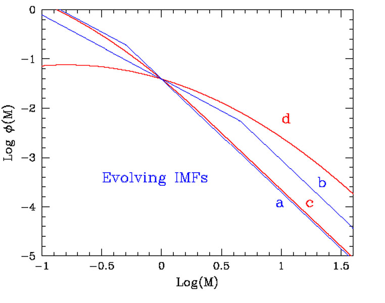Figure 8.3. Examples of evolving IMFs, for a two-slope IMF and a Chabrier-like IMF. Lines a and c represent the local IMF. The other lines show modified IMFs to explore a hypothetical evolution with redshift, with the break mass and the characteristic mass Mc having increased to ~ 4 M, lines b and d respectively for the two-slope and the Chabrier-like IMF. All IMFs have been normalized to have the same value for M = M.