8.4. THE METAL CONTENT OF GALAXY CLUSTERS AND THE IMF SLOPE BETWEEN ~ 1 AND ~ 40 M, AND ABOVE

In its youth, a stellar population generates lots of UV photons, core collapse supernovae and metals that go to enrich the ISM. In its old age, say ~ 12 Gyr later, the same stellar population radiates optical-near-IR light from its ~ 1 M stars, while all more massive stars are dead remnants. The amount of metals (M_X) that are produced by such populations is proportional to the number of massive stars M > ~ 8 M that have undergone a core collapse supernova explosion, whereas the luminosity (e.g., L_B) at t 12 Gyr is proportional to the number of stars with M ~ 1 M. It follows that the metal-mass-to-light ratio M_X / L_B is a measure of the number ratio of massive to ~ M stars, that is, of the IMF slope between ~ 1 and ~ 40 M. Clusters of galaxies offer an excellent opportunity to measure both the light of their dominant stellar populations, and the amount of metals that such populations have produced in their early days. Indeed, most of the light of clusters of galaxies comes from ~ 12 Gyr old, massive ellipticals, and the abundance of metals can be measured both in their stellar populations and in the intracluster medium (ICM). Iron is the element whose abundance can be most reliably measured both in cluster galaxies and in the ICM, but its production is likely to be dominated by Type Ia supernovae whose progenitors are binary stars. As extensively discussed in Chapter 7, a large fraction of the total iron production comes from Type Ia supernovae, and the contribution from CC supernovae is uncertain; therefore the M_Fe / L_B ratio of clusters is less useful to set constraints on the IMF slope between ~ 1 and M > ~ 10 M. For this reason, we focus on oxygen and silicon, whose production is indeed dominated by core collapse supernovae.

Following the notations in Chapter 2, the IMF can be written as:

(8.4)

where a(t, Z) is the relatively slow function of SSP age and metallicity shown in Figure 2.10, multiplied by the bolometric correction shown in Figure 3.1. Thus, the metal-mass-to-light ratio for the generic element "X" can be readily calculated from:

(8.5)

where m_X(M) is the mass of the element X which is produced and ejected by a star of mass M. From stellar population models one has a(12 Gyr, Z) = 2.22 and 3.12, respectively, for Z = Z and 2Z and we adopt a(12 Gyr) = 2.5 in Eq. (8.5). Using the oxygen and silicon yields m_O(M) and m_Si(M) from theoretical nucleosynthesis (cf. 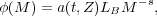Figure 7.5), Equation (8.5) then gives the M_O / L_B and M_Si / L_B metal mass-to-light ratios that are reported in Figure 8.7 as a function of the IMF slope between ~ 1 and ~ 40 M. As expected, the M_O / L_B and M_Si / L_B are extremely sensitive to the IMF slope. The values observed in local clusters of galaxies, from X-ray observations of the ICM and assuming stars are near solar on average, are ~ 0.1 and ~ 0.008 M / L, respectively for oxygen and silicon, as documented in Chapter 10. These empirical values are also displayed in Figure 8.7. A comparison with the calculated values shows that with the Salpeter IMF slope (s = 2.35) the standard explosive nucleosynthesis from core collapse supernovae produces just the right amount of oxygen and silicon to match the observed M_O / L_B and M_Si / L_B ratios in clusters of galaxies, having assumed that most of the B-band light of clusters comes from ~ 12 Gyr old populations. Actually, silicon may be even somewhat overproduced if one allows a ~ 40% contribution from Type Ia supernovae (cf. Figure 7.17).

Figure 8.7. The oxygen and silicon mass-to-light ratios as a function of the IMF slope for a ~ 12 Gyr old, near solar metallicity SSP with oxygen and silicon yields from standard nucleosynthesis calculations. Different lines refer to the different theoretical yields shown in Figure 7.5a,b. The horizontal lines show the uncertainty range of the observed values of these ratios in clusters of galaxies, with central values as reported in Chapter 10, and allowing for a ~ ± 25% uncertainty.

Figure 8.7 also shows that with s = 1.35 such a top heavy IMF would overproduce oxygen and silicon by more than a factor ~ 20. Such a huge variation with s = 1 is actually expected, given that for a near Salpeter slope the typical mass of metal producing stars is ~ 25 M. By the same token, the IMF labelled b in Figure 8.3 would overproduce metals by a factor ~ 4 with respect to a Salpeter-slope IMF (lines a and c ), whereas the IMF labelled d in Figure 8.3 would do so by a factor ~ 20. Thus, under the assumptions that the bulk of the light of local galaxy clusters comes from ~ 12 Gyr old stars, that current stellar theoretical nucleosynthesis is basically correct, and that no large systematic errors affect the reported empirical values of the M_O / L_B and M_Si / L_B ratios, then one can exclude a significant evolution of the IMF with cosmic time, such as for example, one in which the IMF at z ~ 3 would be represented by line b or d in Figure 8.3, and by line a or c at z = 0.

A variable IMF is often invoked as an ad hoc fix to specific discrepancies that may emerge here or there, which however may have other origins. For example, an evolving IMF with redshift has been sometimes invoked to ease a perceived discrepancy between the cosmic evolution of the stellar mass density, and the integral over cosmic time of the star formation rate. In other contexts it has been proposed that the IMF may be different in starbursts as opposed to more steady star formation, or in disks vs. spheroids. Sometimes one appeals to a top-heavy IMF in one context, and then to a bottom-heavy one in another, as if it was possible to have as many IMFs as problems to solve. Honestly, we do not know whether there is one and only one IMF. However, if one subscribes to a different IMF to solve a single problem, then at the same time one should make sure the new IMF does not destroy agreements elsewhere, or conflicts with other astrophysical constraints. While it is perfectly legitimate to contemplate IMF variations from one situation to another, it should be mandatory to explore all consequences of postulated variations, well beyond the specific case one is attempting to fix. This kind of sanitary check is most frequently neglected in the literature appealing to IMF variations. A few examples of such checks have been presented in this chapter.