


2.1.1. The visibility function
"An interferometer is a device for measuring the spatial coherence function" (Clark 1999). This dry statement pretty much captures what interferometry is all about, and the rest of this chapter will try to explain what lies beneath it, how the measured spatial coherence function is turned into images and how properties of the interferometer affect the images. We will mostly abstain from equations here and give a written description instead, however, some equations are inevitable. The issues explained here have been covered in length in the literature, in particular in the first two chapters of Taylor et al. (1999) and in great detail in Thompson et al. (2001).
The basic idea of an interferometer is that the spatial intensity
distribution of electromagnetic radiation produced by an astronomical
object at a particular frequency,
I , can be
reconstructed from the spatial coherence function measured at two points
with the interferometer elements,
V(
, can be
reconstructed from the spatial coherence function measured at two points
with the interferometer elements,
V( 1,
2).
1,
2).
Let the (monochromatic) electromagnetic field arriving at the
observer's location
be denoted by
E(). It is
the sum of all waves emitted by celestial bodies at that particular
frequency. A property of this field is the correlation function at two
points, V(1,
2)
= <E(1)
E*(2)>,
where the superscript * denotes
the complex conjugate.
V(1,
2)
describes how
similar the electromagnetic field measured at two locations is. Think
of two corks thrown into a lake in windy weather. If the corks are
very close together, they will move up and down almost synchronously;
however as their separation increases their motions will become less
and less similar, until they move completely independently when
several meters apart.
Radiation from the sky is largely spatially incoherent, except over very small angles on the sky, and these assumptions (with a few more) then lead to the spatial coherence function
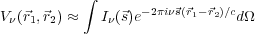 |
(1) |
Here  is the unit
vector pointing towards the source and
d
is the unit
vector pointing towards the source and
d is the surface element of the celestial sphere. The
interesting point of this equation is that it is a function of the
separation and relative orientation of two locations. An
interferometer in Europe will measure the same thing as one in
Australia, provided the separation and orientation of the
interferometer elements are the same. The relevant parameters here are
the coordinates of the antennas when projected onto a plane
perpendicular to the line of sight
(Figure 1). This
plane has the axes u and v, hence it is called the
(u, v)
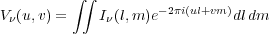
plane. Now let us further introduce units of wavelengths to measure
positions in the (u, v) plane. One then gets
is the surface element of the celestial sphere. The
interesting point of this equation is that it is a function of the
separation and relative orientation of two locations. An
interferometer in Europe will measure the same thing as one in
Australia, provided the separation and orientation of the
interferometer elements are the same. The relevant parameters here are
the coordinates of the antennas when projected onto a plane
perpendicular to the line of sight
(Figure 1). This
plane has the axes u and v, hence it is called the
(u, v)
plane. Now let us further introduce units of wavelengths to measure
positions in the (u, v) plane. One then gets
 |
(2) |
This equation is a Fourier transform between the spatial coherence
function and the (modified) intensity distribution in the sky,
I, and can
be inverted to obtain
I. The
coordinates u
and v are the components of a vector pointing from the origin of the
(u, v) plane to a point in the plane, and describe the
projected separation and orientation of the elements, measured in
wavelengths. The coordinates l and m are direction cosines
towards the astronomical source (or a part thereof). In radio astronomy,
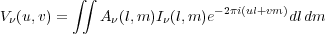
V is called
the visibility function, but a factor,
A, is
commonly included to describe the sensitivity of the interferometer
elements as a function of angle on the sky (the antenna
response 1).
 |
(3) |
The visibility function is the quantity all interferometers measure and which is the input to all further processing by the observer.
 |
Figure 1. Sketch of how a visibility
measurement is obtained from a VLBI
baseline. The source is observed in direction of the line-of-sight
vector, |
We introduced a coordinate system such that the line connecting the interferometer elements, the baseline, is perpendicular to the direction towards the source, and this plane is called the (u, v) plane for obvious reasons. However, the baseline in the (u, v) plane is only a projection of the vector connecting the physical elements. In general, the visibility function will not be the same at different locations in the (u, v) plane, an effect arising from structure in the astronomical source. It is therefore desirable to measure it at as many points in the (u, v) plane as possible. Fortunately, the rotation of the earth continuously changes the relative orientation of the interferometer elements with respect to the source, so that the point given by (u, v) slowly rotates through the plane, and so an interferometer which is fixed on the ground samples various aspects of the astronomical source as the observation progresses. Almost all contemporary radio interferometers work in this way, and the technique is then called aperture synthesis. Furthermore, one can change the observing frequency to move (radially) to a different point in the (u, v) plane. This is illustrated in Figure 2. Note that the visibility measured at (-u, -v) is the complex conjugate of that measured at (u, v), and therefore does not add information. Hence sometimes in plots of (u, v) coverage such as Figure 2, one also plots those points mirrored across the origin. A consequence of this relation is that after 12 h the aperture synthesis with a given array and frequency is complete.
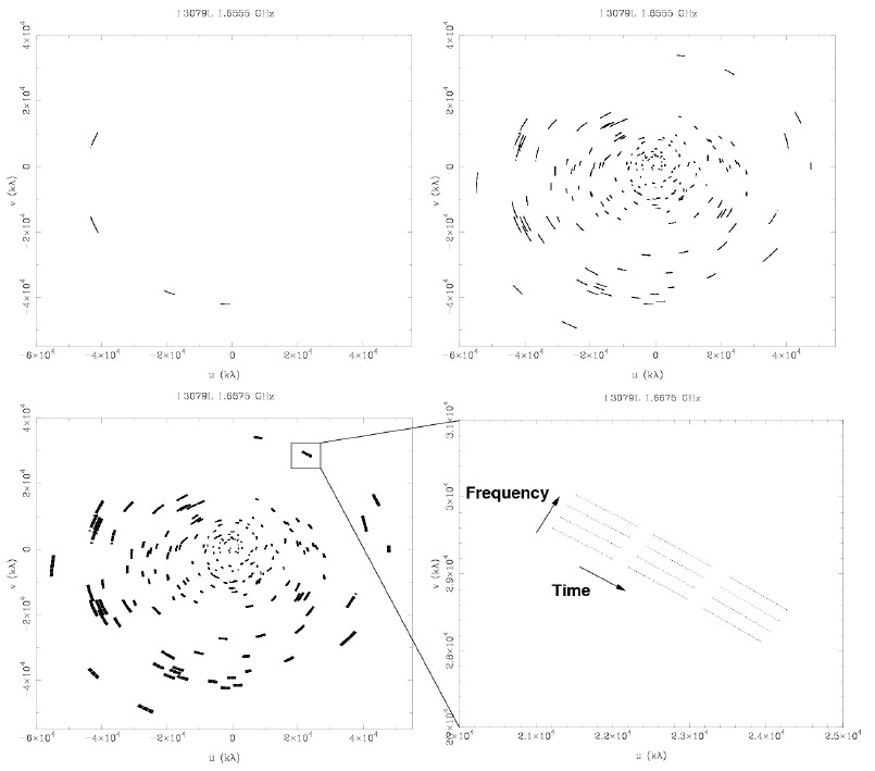 |
Figure 2. Points in the (u, v)
plane sampled during a typical VLBI observation at a frequency of 1.7 GHz
( |
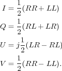
After a typical VLBI observation of one source, the (u, v) coverage will not look too different from the one shown in Figure 2. These are all the data needed to form an image by inverting Equation 3. However, the (u, v) plane has been sampled only at relatively few points, and the purely Fourier-transformed image (the "dirty image") will look poor. This is because the true brightness distribution has been convolved with the instrument's point-spread function (PSF). In the case of aperture synthesis, the PSF B(l, m) is the Fourier transform of the (u, v) coverage:
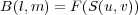 |
(4) |
Here S(u, v)) is unity where measurements have been made, and zero elsewhere. Because the (u, v) coverage is mostly unsampled, B(l,m) has very high artefacts ("sidelobes").
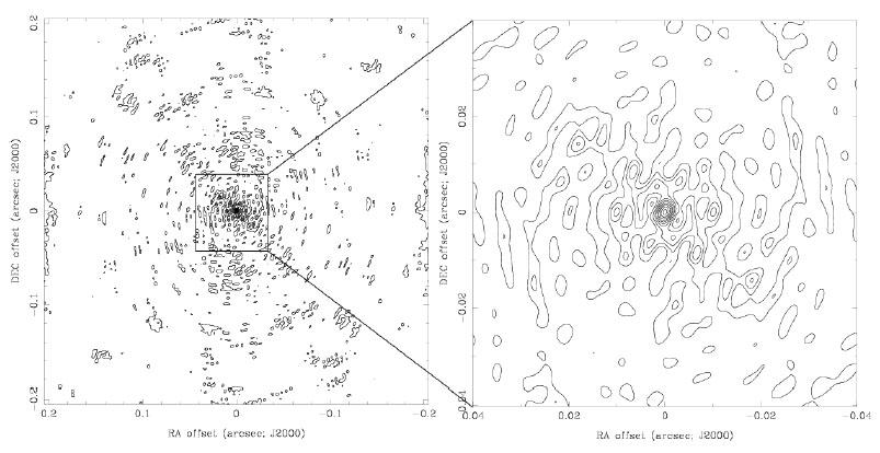 |
Figure 3. The PSF B(l, m) of the (u, v) coverage shown in the bottom left panel of Figure 2. Contours are drawn at 5%, 15%, 25%, ... of the peak response in the image centre. Patches where the response is higher than 5% are scattered all over the image, sometimes reaching 15%. In the central region, the response outside the central peak reaches more than 25%. Without further processing, the achievable dynamic range with this sort of PSF is of the order of a few tens. |
To remove the sidelobes requires to interpolate the visibilities to the empty regions of the (u, v) plane, and the standard method in radio astronomy to do that is the "CLEAN" algorithm.
The CLEAN algorithm (Högbom 1974) is a non-linear, iterative mechanism to rid interferometry images of artefacts caused by insufficient (u, v) coverage. Although a few varieties exist the basic structure of all CLEAN implementations is the same:
 l,
mi +
m).
l,
mi +
m).
 << 1 and keep the residual: R(l, m)
= I'(l, m) -
c
B(l +
l,
m + m)
<< 1 and keep the residual: R(l, m)
= I'(l, m) -
c
B(l +
l,
m + m)
I'(li, mi)) as a delta
component to the "clean image" and start over again.
CLEAN can be stopped when the sidelobes of the sources in the residual image are much lower than the image noise. A corollary of this is that in the case of very low signal-to-noise ratios CLEAN will essentially have no effect on the image quality, because the sidelobes are below the noise limit introduced by the receivers in the interferometer elements. The "clean image" is iteratively build up out of delta components, and the final image is formed by convolving it with the "clean beam". The clean beam is a two-dimensional Gaussian which is commonly obtained by fitting a Gaussian to the centre of the dirty beam image. After the convolution the residual image is added.
 |
Figure 4. Illustration of the effects of the CLEAN algorithm. Left panel: The Fourier transform of the visibilities already used for illustration in Figures 2 and 3. The image is dominated by artefacts arising from the PSF of the interferometer array. The dynamic range of the image (the image peak divided by the rms in an empty region) is 25. Right panel: The "clean image", made by convolving the model components with the clean beam, which in this case has a size of 3.0 × 4.3 mas. The dynamic range is 144. The contours in both panels start at 180 µJy and increase by factors of two. |
The way in which images are formed in radio interferometry may seem difficult and laborious (and it is), but it also adds great flexibility. Because the image is constructed from typically thousands of interferometer measurements one can choose to ignore measurements from, e.g., the longest baselines to emphasize sensitivity to extended structure. Alternatively, one can choose to weight down or ignore short spacings to increase resolution. Or one can convolve the clean model with a Gaussian which is much smaller than the clean beam, to make a clean image with emphasis on fine detail ("superresolution").
2.1.5. Generating a visibility measurement
The previous chapter has dealt with the fundamentals of interferometry and image reconstruction. In this chapter we will give a brief overview about more technical aspects of VLBI observations and the signal processing involved to generate visibility measurements.
It may have become clear by now that an interferometer array really is only a collection of two-element interferometers, and only at the imaging stage is the information gathered by the telescopes combined. In an array of N antennas, the number of pairs which can be formed is N(N - 1) / 2, and so an array of 10 antennas can measure the visibility function at 45 locations in the (u, v) plane simultaneously. Hence, technically, obtaining visibility measurements with a global VLBI array consisting of 16 antennas is no more complex than doing it with a two-element interferometer - it is just logistically more challenging.
Because VLBI observations involve telescopes at widely separated locations (and can belong to different institutions), VLBI observations are fully automated. The entire "observing run" (a typical VLBI observations lasts around 12 h) including setting up the electronics, driving the antenna to the desired coordinates and recording the raw antenna data on tape or disk, is under computer control and requires no interaction by the observer. VLBI observations generally are supervised by telescope operators, not astronomers.
It should be obvious that each antenna needs to point towards the direction of the source to be observed, but as VLBI arrays are typically spread over thousands of kilometres, a source which just rises at one station can be in transit at another 2. Then the electronics need to be set up, which involves a very critical step: tuning the local oscillator. In radio astronomy, the signal received by the antenna is amplified many times (in total the signal is amplified by factors of the order of 108 to 1010), and to avoid receiver instabilities the signal is "mixed down" to much lower frequencies after the first amplification. The mixing involves injecting a locally generated signal (the local oscillator, or LO, signal) into the signal path with a frequency close to the observing frequency. This yields the signal at a frequency which is the difference between the observing frequency and the LO frequency (see, e.g., Rohlfs 1986 for more details). The LO frequency must be extremely stable (1 part in 1015 per day or better) and accurately known (to the sub-Hz level) to ensure that all antennas observe at the same frequency. Interferometers with connected elements such as the VLA or ATCA only need to generate a single LO the output of which can be sent to the individual stations, and any variation in its frequency will affect all stations equally. This is not possible in VLBI, and so each antenna is equipped with a maser (mostly hydrogen masers) which provides a frequency standard to which the LO is phase-locked. After downconversion, the signal is digitized at the receiver output and either stored on tape or disk, or, more recently, directly sent to the correlator via fast network connections ("eVLBI").
The correlator is sometimes referred to as the "lens" of VLBI observations, because it produces the visibility measurements from the electric fields sampled at the antennas. The data streams are aligned, appropriate delays and phases introduced and then two operations need to be performed on segments of the data: the cross-multiplication of each pair of stations and a Fourier transform, to go from the temporal domain into the spectral domain. Note that Eq.3 is strictly valid only at a particular frequency. Averaging in frequency is a source of error, and so the observing band is divided into frequency channels to reduce averaging, and the VLBI measurand is a cross-power spectrum.
The cross-correlation and Fourier transform can be interchanged, and correlator designs exists which carry out the cross-correlation first and then the Fourier transform (the "lag-based", or "XF", design such as the MPIfR's Mark IV correlator and the ATCA correlator), and also vice versa (the "FX" correlator such as the VLBA correlator). The advantages and disadvantages of the two designs are mostly in technical details and computing cost, and of little interest to the observer once the instrument is built. However, the response to spectral lines is different. In a lag-based correlator the signal is Fourier transformed once after cross-correlation, and the resulting cross-power spectrum is the intrinsic spectrum convolved with the sinc function. In a FX correlator, the input streams of both interferometer elements are Fourier transformed which includes a convolution with the sinc function, and the subsequent cross-correlation produces a spectrum which is convolved with the square of the sinc function. Hence the FX correlator has a finer spectral resolution and lower sidelobes (see Romney 1999).
The vast amount of data which needs to be processed in interferometry observations has always been processed on purpose-built computers (except for the very observations where bandwidths of the order of several hundred kHz were processed on general purpose computers). Only recently has the power of off-the-shelf PCs reached a level which makes it feasible to carry out the correlation in software. Deller et al. (2007) describe a software correlator which can efficiently run on a cluster of PC-architecture computers. Correlation is an "embarrassingly parallel" problem, which can be split up in time, frequency, and by baseline, and hence is ideally suited to run in a cluster environment.
The result of the correlation stage is a set of visibility measurements. These are stored in various formats along with auxiliary information about the array such as receiver temperatures, weather information, pointing accuracy, and so forth. These data are sent to the observer who has to carry out a number of calibration steps before the desired information can be extracted.
2.2. Sources of error in VLBI observations
VLBI observations generally are subject to the same problems as observations with connected-element interferometers, but the fact that the individual elements are separated by hundreds and thousands of kilometres adds a few complications.
The largest source of error in typical VLBI observations are phase errors introduced by the earth's atmosphere. Variations in the atmosphere's electric properties cause varying delays of the radio waves as they travel through it. The consequence of phase errors is that the measured flux of individual visibilities will be scattered away from the correct locations in the image, reducing the SNR of the observations or, in fact, prohibiting a detection at all. Phase errors arise from tiny variations in the electric path lengths from the source to the antennas. The bulk of the ionospheric and tropospheric delays is compensated in correlation using atmospheric models, but the atmosphere varies on very short timescales so that there are continuous fluctuations in the measured visibilities.
At frequencies below 5 GHz changes in the electron content (TEC) of the ionosphere along the line of sight are the dominant source of phase errors. The ionosphere is the uppermost part of the earth's atmosphere which is ionised by the sun, and hence undergoes diurnal and seasonal changes. At low GHz frequencies the ionosphere's plasma frequency is sufficiently close to the observing frequency to have a noticeable effect. Unlike tropospheric and most other errors, which have a linear dependence on frequency, the impact of the ionosphere is proportional to the inverse of the frequency squared, and so fades away rather quickly as one goes to higher frequencies. Whilst the TEC is regularly monitored 3 and the measurements can be incorporated into the VLBI data calibration, the residual errors are still considerable.
At higher frequencies changes in the tropospheric water vapour content have the largest impact on radio interferometry observations. Water vapour 4 does not mix well with air and thus the integrated amount of water vapour along the line of sight varies considerably as the wind blows over the antenna. Measuring the amount of water vapour along the line of sight is possible and has been implemented at a few observatories (Effelsberg, CARMA, Plateau de Bure), however it is difficult and not yet regularly used in the majority of VLBI observations.
Compact arrays generally suffer less from atmospheric effects because most of the weather is common to all antennas. The closer two antennas are together, the more similar the atmosphere is along the lines of sight, and the delay difference between the antennas decreases.
Other sources of error in VLBI observations are mainly uncertainties in the geometry of the array and instrumental errors. The properties of the array must be accurately known in correlation to introduce the correct delays. As one tries to measure the phase of an electromagnetic wave with a wavelength of a few centimetres, the array geometry must be known to a fraction of that. And because the earth is by no means a solid body, many effects have to be taken into account, from large effects like precession and nutation to smaller effects such as tectonic plate motion, post-glacial rebound and gravitational delay. For an interesting and still controversial astrophysical application of the latter, see Fomalont and Kopeikin (2003). For a long list of these effects including their magnitudes and timescales of variability, see Walker (1999).
2.3. The problem of phase calibration: self-calibration
Due to the aforementioned errors, VLBI visibilities directly from the correlator will never be used to make an image of astronomical sources. The visibility phases need to be calibrated in order to recover the information about the source's location and structure. However, how does one separate the unknown source properties from the unknown errors introduced by the instrument and atmosphere? The method commonly used to do this is called self-calibration and works as follows.
In simple words, in self-calibration one uses a model of the source (if a model is not available a point source is used) and tries to find phase corrections for the antennas to make the visibilities comply with that model. This won't work perfectly unless the model was a perfect representation of the source, and there will be residual, albeit smaller, phase errors. However the corrected visibilities will allow one to make an improved source model, and one can find phase corrections to make the visibilities comply with that improved model, which one then uses to make an even better source model. This process is continued until convergence is reached.
The assumption behind self-calibration is that the errors in the visibility phases, which are baseline-based quantities, can be described as the result of antenna-based errors. Most of the errors described in Sec 2.2 are antenna-based: e.g. delays introduced by the atmosphere, uncertainties in the location of the antennas, and drifts in the electronics all are antenna-based. The phase error of a visibility is the combination of the antenna-based phase errors 5. Since the number of unknown station phase errors is less than the number of visibilities, there is additional phase information which can be used to determine the source structure.
However, self-calibration contains some traps. The most important is making a model of the source which is usually accomplished by making a deconvolved image with the CLEAN algorithm. If a source has been observed during an earlier epoch and the structural changes are expected to be small, then one can use an existing model for a start. If in making that model one includes components which are not real (e.g., by cleaning regions of the image which in fact do not contain emission) then they will be included in the next iteration of self-calibration and will re-appear in the next image. Although it is not easy to generate fake sources or source parts which are strong, weaker source structures are easily affected. The authors have witnessed a radio astronomy PhD student producing a map of a colleague's name using a data set of pure noise, although the SNR was of the order of only 3.
It is also important to note that for self-calibration the SNR of the visibilities needs to be of the order of 5 or higher within the time it takes the fastest error component to change by a few tens of degrees ("atmospheric coherence time") (Cotton 1995). Thus the integration time for self-calibration usually is limited by fluctuations in the tropospheric water vapour content. At 5 GHz, one may be able to integrate for 2 min without the atmosphere changing too much, but this can drop to as little as 30 s at 43 GHz. Because radio antennas used for VLBI are less sensitive at higher frequencies observations at tens of GHz require brighter and brighter sources to calibrate the visibility phases. Weak sources well below the detection threshold within the atmospheric coherence time can only be observed using phase referencing (see Sec. 2.3.1.)
Another boundary condition for successfully self-calibration is that for a given number of array elements the source must not be too complex. The more antennas, the better because the ratio of number of constraints to number of antenna gains to be determined goes as N/2 (The number of constraints is the number of visibilities, N(N - 1) / 2. The number of gains is the number of stations, N, minus one, because the phase of one station is a free parameter and set to zero). Thus self-calibration works very well at the VLA, even with complex sources, whereas for an east-west interferometer with few elements such as the ATCA, self-calibration is rather limited. In VLBI observations, however, the sources are typically simple enough to make self-calibration work even with a modest number (N > 5) of antennas.
It is possible to obtain phase-calibrated visibilities without self-calibration by measuring the phase of a nearby, known calibrator. The assumption is that all errors for the calibrator and the target are sufficiently similar to allow calibration of the target with phase corrections derived from the calibrator. While this assumption is justified for the more slowly varying errors such as clock errors and array geometry errors (provided target and calibrator are close), it is only valid under certain circumstances when atmospheric errors are considered. The critical ingredients in phase referencing observations are the target-calibrator separation and the atmospheric coherence time. The separation within which the phase errors for the target and calibrator are considered to be the same is called the isoplanatic patch, and is of the order of a few degrees at 5 GHz. The switching time must be shorter than the atmospheric coherence time to prevent undersampling of the atmospheric phase variations. At high GHz frequencies this can result in observing strategies where one spends half the observing time on the calibrator.
Phase-referencing not only allows one to observe sources too weak for self-calibration, but it also yields precise astrometry for the target relative to the calibrator. A treatment of the attainable accuracy can be found in Pradel et al. (2006).
The polarization of radio emission can yield insights into the strength and orientation of magnetic fields in astrophysical objects and the associated foregrounds. As a consequence and because the calibration has become easier and more streamlined it has become increasingly popular in the past 10 years to measure polarization.
Most radio antennas can record two orthogonal polarizations, conventionally in the form of dual circular polarization. In correlation, one can correlate the right-hand circular polarization signal (RCP) of one antenna with the left-hand circular polarization (LCP) of another and vice versa, to obtain the cross-polarization products RL and LR. The parallel-hand circular polarization cross-products are abbreviated as RR and LL. The four correlation products are converted into the four Stokes parameters in the following way:
 |
(5) |
From the Stokes images one can compute images of polarized intensity and polarization angle.
Most of the calibration in polarization VLBI observations is identical to conventional observations, where one either records only data in one circular polarization or does not form the cross-polarization data at the correlation stage. However, two effects need to be taken care of, the relative phase relation between RCP and LCP and the leakage of emission from RCP and LCP into the cross-products.
The relative phase orientation of RCP and LCP needs to be calibrated to obtain the absolute value for the electric vector position angle (EVPA) of the polarized emission in the source. This is usually accomplished by observing a calibrator which is known to have a stable EVPA with a low-resolution instrument such as a single dish telescope or a compact array.
Calibration of the leakage is more challenging. Each radio telescope has polarization impurities arising from structural asymmetries and errors in manufacturing, resulting in "leakage" of emission from one polarization to the other. The amount of leakage typically is of the order of a few percent and thus is of the same order as the typical degree of polarization in the observed sources and so needs to be carefully calibrated. The leakage is a function of frequency but can be regarded as stable over the course of a VLBI observation.
Unfortunately, sources which are detectable with VLBI are extremely small and hence mostly variable. It is therefore not possible to calibrate the leakage by simply observing a polarization calibrator, and the leakage needs to be calibrated by every observer. At present the calibration scheme exploits the fact that the polarized emission arising from leakage does not change its position angle in the course of the observations. The EVPA of the polarized emission coming from the source, however, will change with respect to the antenna and its feed horns, because most antennas have alt-azimuth mounts and so the source seems to rotate on the sky as the observation progresses 6. One can think of this situation as the sum of two vectors, where the instrumental polarization is a fixed vector and the astronomical polarization is added to this vector and rotates during the observation. Leakage calibration is about separating these two contributions, by observing a strong source at a wide range of position angles. The method is described in Leppänen et al. (1995), and a more detailed treatment of polarization VLBI is given by Kemball (1999).
In general a set of visibility measurements consists of cross-power spectra. If a continuum source has been targeted, the number of spectral points is commonly of the order of a few tens. If a spectral line has been observed, the number of channels can be as high as a few thousand, and is limited by the capabilities of the correlator. The high brightness temperatures (Section 3.1.3) needed to yield a VLBI detection restrict observations to masers, or relatively large absorbers in front of non-thermal continuum sources. The setup of frequencies requires the same care as for short baseline interferometry, but an additional complication is that the antennas have significant differences in their Doppler shifts towards the source. See Westpfahl (1999), Rupen (1999), and Reid et al. (1999) for a detailed treatment of spectral-line interferometry and VLBI.
If pulsars are to be observed with a radio interferometer it is desirable to correlate only those times where a pulse is arriving (or where it is absent, Stappers et al. 1999). This is called pulsar gating and is an observing mode available at most interferometers.
The equations in Sec. 2.1 are strictly correct only
for a single frequency and single points in time, but radio telescopes
must observe a finite bandwidth, and in correlation a finite
integration time must be used, to be able to detect objects. Hence a
point in the (u, v) plane always represents the result of
averaging across a bandwidth,
, and over a time interval,
 (the points in Fig. 2 actually represent a
continuous frequency band in the radial direction and a continuous
observation in the time direction).
(the points in Fig. 2 actually represent a
continuous frequency band in the radial direction and a continuous
observation in the time direction).
The errors arising from averaging across the bandwidth are referred to
as bandwidth smearing, because the effect is similar to chromatic
aberration in optical systems, where the light from one single point
of an object is distributed radially in the image plane. In radio
interferometry, the images of sources away from the observing centre
are smeared out in the radial direction, reducing the signal-to-noise
ratio. The effect of bandwidth smearing increases with the fractional
bandwidth,
/
, the square root of the
distance to the observing centre, (l2 +
m2)1/2, and with 1 /
 b, where
b is the FWHM
of the synthesized beam. Interestingly, however, the dependencies of
of the fractional bandwidth
and of
b cancel one
another, and so for any given array and
bandwidth, bandwidth smearing is independent of
(see
Thompson et
al. 2001).
The effect can be avoided if the observing
band is subdivided into a sufficiently large number of frequency
channels for all of which one calculates the locations in the (u,
v)
plane separately. This technique is sometimes deliberately chosen to
increase the (u, v) coverage, predominantly at low
frequencies where the fractional bandwidth is large. It is then called
multi-frequency synthesis.
b, where
b is the FWHM
of the synthesized beam. Interestingly, however, the dependencies of
of the fractional bandwidth
and of
b cancel one
another, and so for any given array and
bandwidth, bandwidth smearing is independent of
(see
Thompson et
al. 2001).
The effect can be avoided if the observing
band is subdivided into a sufficiently large number of frequency
channels for all of which one calculates the locations in the (u,
v)
plane separately. This technique is sometimes deliberately chosen to
increase the (u, v) coverage, predominantly at low
frequencies where the fractional bandwidth is large. It is then called
multi-frequency synthesis.
By analogy, the errors arising from time averaging are called time
smearing, and they smear out the images approximately tangentially to
the (u, v) ellipse. It occurs because each point in the
(u, v) plane
represents a measurement during which the baseline vector rotated
through  E
, where
E is
the angular velocity
of the earth. Time smearing also increases as a function of
(l2 + m2)1/2 and can be
avoided if is chosen small
enough for the desired field of view.
E
, where
E is
the angular velocity
of the earth. Time smearing also increases as a function of
(l2 + m2)1/2 and can be
avoided if is chosen small
enough for the desired field of view.
VLBI observers generally are concerned with fields of view (FOV) of no more than about one arcsecond, and consequently most VLBI observers are not particularly bothered by wide field effects. However, wide-field VLBI has gained momentum in the last few years as the computing power to process finely time- and bandwidth-sampled data sets has become widely available. Recent examples of observations with fields of view of 1' or more are reported on in McDonald et al. (2001), Garrett et al. (2001), Garrett et al. (2005), Lenc and Tingay (2006) and Lenc et al. (2006). The effects of primary beam attenuation, bandwidth smearing and time smearing on the SNR of the observations can be estimated using the calculator at http://astronomy.swin.edu.au/~elenc/Calculators/wfcalc.php.
In the quest for angular resolution VLBI helps to optimize one part of
the equation which approximates the separation of the finest details
an instrument is capable of resolving,
=
 / D . In VLBI,
D approaches the diameter of the earth, and larger instruments are
barely possible, although "space-VLBI" can extend an array beyond
earth. However, it is straightforward to attempt to decrease
to push the resolution further up.
/ D . In VLBI,
D approaches the diameter of the earth, and larger instruments are
barely possible, although "space-VLBI" can extend an array beyond
earth. However, it is straightforward to attempt to decrease
to push the resolution further up.
However, VLBI observations at frequencies above 20 GHz
( = 15 mm) become
progressively harder towards higher
frequencies. Many effects contribute to the difficulties at mm
wavelengths: the atmospheric coherence time is shorter than one
minute, telescopes are less efficient, receivers are less sensitive,
sources are weaker than at cm wavelengths, and tropospheric water
vapour absorbs the radio emission. All of these effects limit mm VLBI
observations to comparatively few bright continuum sources or sources
hosting strong masers. Hence also the number of possible phase
calibrators for phase referencing drops. Nevertheless VLBI
observations at 22 GHz (13 mm) , 43 GHz
(
 7 mm) and
86 GHz (
3 mm) are routinely carried out with the
world's VLBI arrays. For example, of all projects observed in 2005 and
2006 with the VLBA, 16% were made at 22 GHz, 23% at 43 GHz,
and 4% at 86 GHz 7.
7 mm) and
86 GHz (
3 mm) are routinely carried out with the
world's VLBI arrays. For example, of all projects observed in 2005 and
2006 with the VLBA, 16% were made at 22 GHz, 23% at 43 GHz,
and 4% at 86 GHz 7.
Although observations at higher frequencies are experimental, a
convincing demonstration of the feasibility of VLBI at wavelengths
shorter than 3 mm was made at 2 mm (147 GHz) in 2001 and 2002
(Krichbaum et al. 2002a,
Greve
et al. 2002).
These first 2 mm-VLBI experiments
resulted in detections of about one dozen quasars on the short
continental and long transatlantic baselines
(Krichbaum et al. 2002a).
In an experiment in April 2003 at 1.3 mm
(230 GHz) a number of sources was detected on the 1150 km long
baseline between Pico Veleta and Plateau de Bure
(Krichbaum et al. 2004).
On the 6.4 G long
transatlantic baseline between Europe and Arizona, USA fringes for the
quasar 3C 454.3 were clearly seen. This detection marks a new record in
angular resolution in Astronomy (size < 30 µas). It
indicates the
existence of ultra compact emission regions in AGN even at the highest
frequencies (for 3C 454.3 at z = 0.859, the rest frame frequency is
428 GHz). So far, no evidence for a reduced brightness temperature of
the VLBI-cores at mm wavelengths was found
(Krichbaum et al. 2004).
These are the astronomical observations
with the highest angular resolution possible today at any wavelength.
2.9. The future of VLBI: eVLBI, VLBI in space, and the SKA
One of the key drawbacks of VLBI observations has always been that the raw antenna signals are recorded and the visibilities formed only later when the signals are combined in the correlator. Thus there has never been an immediate feedback for the observer, who has had to wait several weeks or months until the data are received for investigation. With the advent of fast computer networks this has changed in the last few years. First small pieces of raw data were sent from the antennas to the correlator, to check the integrity of the VLBI array, then data were directly streamed onto disks at the correlator, then visibilities were produced in real-time from the data sent from the antennas to the correlator. A brief description of the transition from tape-based recording to real-time correlation of the European VLBI Network (EVN) is given in Szomoru et al. (2004). The EVN now regularly performs so-called "eVLBI" observing runs which is likely to be the standard mode of operation in the near future. The Australian Long Baseline Array (LBA) completed a first eVLBI-only observing run in March 2007 8.
It has been indicated in Sec. 2.8 that resolution can be increased not only by observing at higher frequencies with ground-based arrays but also by using a radio antenna in earth orbit. This has indeed been accomplished with the Japanese satellite "HALCA" (Highly Advanced Laboratory for Communications and Astronomy, Hirabayashi et al. 2000) which was used for VLBI observations at 1.6 GHz, 5 GHz and 22 GHz (albeit with very low sensitivity) between 1997 and 2003. The satellite provided the collecting area of an 8 m radio telescope and the sampled signals were directly transmitted to ground-based tracking stations. The satellite's elliptical orbit provided baselines between a few hundred km and more than 20000 km, yielding a resolution of up to 0.3 mas ( Dodson et al. 2006, Edwards and Piner 2002). Amazingly, although HALCA only provided left-hand circular polarization, it has been used successfully to observe polarized emission (e.g., Kemball et al. 2000, Bach et al. 2006a). But this was only possible because the ground array observed dual circular polarization. Many of the scientific results from VSOP are summarized in two special issues of Publications of the Astronomical Society of Japan (PASJ, Vol. 52, No. 6, 2000 and Vol. 58, No. 2, 2006). The successor to HALCA, ASTRO-G, is under development and due for launch in 2012. It will have a reflector with a diameter of 9 m and receivers for observations at 8 GHz, 22 GHz, and 43 GHz.
The Russian mission RadioAstron is a similar project to launch a 10 m radio telescope into a high apogee orbit. It will carry receivers for frequencies between 327 MHz and 25 GHz, and is due for launch in October 2008.
The design goals for the Square Kilometre Array (SKA), a large, next-generation radio telescope built by an international consortium, include interferometer baselines of at least 3000 km. At the same time, the design envisions the highest observing frequency to be 25 GHz, and so one would expect a maximum resolution of around 1 mas. However, most of the baselines will be shorter than 3000 km, and so a weighted average of all visibilities will yield a resolution of a few mas, and of tens of mas at low GHz frequencies. The SKA's resolution will therefore be comparable to current VLBI arrays. Its sensitivity, however, will be orders of magnitude higher (sub-µJy in 1 h). The most compelling consequence of this is that the SKA will allow one to observe thermal sources with brightness temperatures of the order of a few hundred Kelvin with a resolution of a few mas. Current VLBI observations are limited to sources with brightness temperatures of the order of 106 K and so to non-thermal radio sources and coherent emission from masers. With the SKA one can observe star and black hole formation throughout the universe, stars, water masers at significant redshifts, and much more. Whether or not the SKA can be called a VLBI array in the original sense (an array of isolated antennas the visibilities of which are produced later on) is a matter of taste: correlation will be done in real time and the local oscillator signals will be distributed from the same source. Still, the baselines will be "very long" when compared to 20th century connected-element interferometers. A short treatment of "VLBI with the SKA" can be found in Carilli (2005). Comprehensive information about the current state of the SKA is available on the aforementioned web page; prospects of the scientific outcomes of the SKA are summarized in Carilli and Rawlings (2004); and engineering aspects are treated in Hall (2005).
2.10. VLBI arrays around the world and their capabilities
This section gives an overview of presently active VLBI arrays which are available for all astronomers and which are predominantly used for astronomical observations. Antennas of these arrays are frequently used in other array's observations, to either add more long baselines or to increase the sensitivity of the observations. Joint observations including the VLBA and EVN antennas are quite common; also observations with the VLBA plus two or more of the phased VLA, the Green Bank, Effelsberg and Arecibo telescopes (then known as the High Sensitivity Array) have recently been made easier through a common application process. Note that each of these four telescopes has more collecting area than the VLBA alone, and hence the sensitivity improvement is considerable.
| Square Kilometre Array | http://www.skatelescope.org |
| High Sensitivity Array | http://www.nrao.edu/HSA |
| European VLBI Network | http://www.evlbi.org |
| Very Long Baseline Array | http://www.vlba.nrao.edu |
| Long Baseline Array | http://www.atnf.csiro.au/vlbi |
| VERA | http://veraserver.mtk.nao.ac.jp/outline/index-e.html |
| GMVA | http://www.mpifr-bonn.mpg.de/div/vlbi/globalmm |
2.10.1 The European VLBI Network (EVN)
The EVN is a collaboration of 14 institutes in Europe, Asia, and South Africa and was founded in 1980. The participating telescopes are used in many independent radio astronomical observations, but are scheduled three times per year for several weeks together as a VLBI array. The EVN provides frequencies in the range of 300 MHz to 43 GHz, though due to its inhomogeneity not all frequencies can be observed at all antennas. The advantage of the EVN is that it includes several relatively large telescopes such as the 76 m Lovell telescope, the Westerbork array, and the Effelsberg 100 m telescope, which provide high sensitivity. Its disadvantages are a relatively poor frequency agility during the observations, because not all telescopes can change their receivers at the flick of a switch. EVN observations are mostly correlated on the correlator at the Joint Institute for VLBI in Europe (JIVE) in Dwingeloo, the Netherlands, but sometimes are processed at the Max-Planck-Institute for Radio Astronomy in Bonn, Germany, or the National Radio Astronomy Observatory in Socorro, USA.
2.10.2. The U.S. Very Long Baseline Array (VLBA)
The VLBA is a purpose-built VLBI array across the continental USA and islands in the Caribbean and Hawaii. It consists of 10 identical antennas with a diameter of 25 m, which are remotely operated from Socorro, New Mexico. The VLBA was constructed in the early 1990s and began full operations in 1993. It provides frequencies between 300 MHz and 86 GHz at all stations (except two which are not worth equipping with 86 GHz receivers due to their humid locations). Its advantages are excellent frequency agility and its homogeneity, which makes it very easy to use. Its disadvantages are its comparatively small antennas, although the VLBA is frequently used in conjunction with the phased VLA and the Effelsberg and Green Bank telescopes.
2.10.3. The Australian Long Baseline Array (LBA)
The LBA consists of six antennas in Ceduna, Hobart, Parkes, Mopra, Narrabri, and Tidbinbilla. Like the EVN it has been formed from existing antennas and so the array is inhomogeneous. Its frequency range is 1.4 GHz to 22 GHz, but not all antennas can observe at all available frequencies. Stretched out along Australia's east coast, the LBA extends in a north-south direction which limits the (u, v) coverage. Nevertheless, the LBA is the only VLBI array which can observe the entire southern sky, and the recent technical developments are remarkable: the LBA is at the forefront of development of eVLBI and at present is the only VLBI array correlating all of its observations using the software correlator developed by Deller et al. (2007) on a computer cluster of the Swinburne Centre for Astrophysics and Supercomputing.
2.10.4. The Korean VLBI Network (KVN)
The KVN is a dedicated VLBI network consisting of three antennas which currently is under construction in Korea. It will be able to observe at up to four widely separated frequencies (22 GHz, 43 GHz, 86 GHz, and 129 GHz), but will also be able to observe at 2.3 GHz and 8.4 GHz. The KVN has been designed to observe H2O and SiO masers in particular and can observe these transitions simultaneously. Furthermore, the antennas can slew quickly for improved performance in phase-referencing observations.
2.10.5. The Japanese VERA network
VERA (VLBI Exploration of Radio Astrometry) is a purpose-built VLBI network of four antennas in Japan. The scientific goal is to measure the annual parallax towards galactic masers (H2O masers at 22 GHz and SiO masers at 43 GHz), to construct a map of the Milky Way. Nevertheless, VERA is open for access to carry out any other observations. VERA can observe two sources separated by up to 2.2° simultaneously, intended for an extragalactic reference source and for the galactic target. This observing mode is a significant improvement over the technique of phase-referencing where the reference source and target are observed in turn. The positional accuracy is expected to reach 10 µas, and recent results seem to reach this (Hirota et al. 2007b). VERA's frequency range is 2.3 GHz to 43 GHz.
2.10.6. The Global mm-VLBI Array (GMVA)
The GMVA is an inhomogeneous array of 13 radio telescopes capable of observing at a frequency of 86 GHz. Observations with this network are scheduled twice a year for about a week. The array's objective is to provide the highest angular resolution on a regular schedule.
1 The fields of view in VLBI observations are
typically so small that the dependence of (l,m) can be safely
ignored.
A can then
be set to unity and disappears.
Back.
2 This can be neatly observed with the VLBA's webcam images available at http://www.vlba.nrao.edu/sites/SITECAM/allsites.shtml. The images are updated every 5 min. Back.
3 http://iono.jpl.nasa.gov Back.
4 note that clouds do not primarily consist of water vapour, but of condensated water in droplets. Back.
5 Baseline-based errors exist, too, but are far less important, see Cornwell and Fomalont (1999) for a list. Back.
6 The 26 m antenna at the Mount Pleasant Observatory near Hobart, Australia, has a parallactic mount and thus there is no field rotation. Back.
7 e.g., ftp://ftp.aoc.nrao.edu/pub/cumvlbaobs.txt Back.
8 http://www.atnf.csiro.au/vlbi/evlbi/ Back.
 /
c. At each station, the signals
are intercepted with antennas, amplified, and then mixed down to a low
frequency where they are further amplified and sampled. The essential
difference between a connected-element interferometer and a VLBI array
is that each station has an independent local oscillator, which
provides the frequency normal for the conversion from the observed
frequency to the recorded frequency. The sampled signals are written
to disk or tape and shipped to the correlator. At the correlator, the
signals are played back, the geometric delay
/
c. At each station, the signals
are intercepted with antennas, amplified, and then mixed down to a low
frequency where they are further amplified and sampled. The essential
difference between a connected-element interferometer and a VLBI array
is that each station has an independent local oscillator, which
provides the frequency normal for the conversion from the observed
frequency to the recorded frequency. The sampled signals are written
to disk or tape and shipped to the correlator. At the correlator, the
signals are played back, the geometric delay