


The fundamental driver of progress in astronomy is through observations. The advent of large galaxy surveys, either wide spectroscopic surveys probing the nearby Universe (e.g., SDSS) or narrower surveys using photometric redshifts and often in the infrared domain (e.g., with Spitzer and Herschel) to probe distant galaxies in the optical and near-infrared domains, has led to formidable progress in understanding galaxy formation. Nevertheless, it is difficult to link the galaxies we see at high redshift with the ones we see in local Universe, and one is prone to Malmquist bias, as well as aperture and other selection effects.
Several simulation techniques have been developed to be able to link galaxies from the past to the present, and to obtain a statistical view of the variety of the evolution histories of galaxies, in terms of star formation, stellar mass assembly and halo mass assembly.
Given current computational constraints, it is impossible to achieve the sub-parsec or finer resolution needed to adequately model star formation and accretion onto black holes in a cosmological simulation. Theorists have invented a swindle, wherein the complex processes of star formation and accretion onto SMBH are hidden inside a black box called "sub-grid physics" that can be tagged onto a large-scale simulation. In SAMs, galaxies are "painted" on halos built from halo merger trees or detected in cosmological dissipationless (dark matter only) simulations. The former (see Fig. 10) produce the mass assembly history (MAH) of halos with the condition that they end up in a halo of mass M0 at epoch z0 (usually z0 = 0). The branches are drawn from random samplings given the known conditional probabilities arising from extensions (Bower 1991, Lacey & Cole 1993) and modifications of the (Press & Schechter 1974) formalism. Halo merger trees have the advantage of being rapid to compute, but lack positional information. Cosmological simulations, with up to 108 particles, are becoming increasingly common, but are intensive to process, in particular to detect halos (Knebe et al. 2011 and references therein) and subhalos (Onions et al. 2012 and references therein) and build halo merger trees.
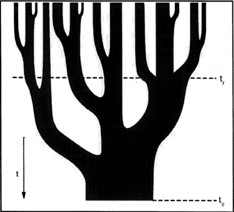 |
Figure 10. Illustration of halo merger tree (Lacey & Cole 1993) showing the progenitors of a halo selected at time t0 |
Once the halo MAH is identified, one follows the branches of the tree from past to present, to build galaxies. The galaxy formation recipe includes several ingredients:
 = cst
mgas / tdyn, where
tdyn is a measure of the dynamical time of the galaxy.
= cst
mgas / tdyn, where
tdyn is a measure of the dynamical time of the galaxy.
An advantage of SAMs is that it is easy to gauge the importance of various physical processes by seeing how the outcome is changed when a process is turned off in the SAM.
Present-day SAMs are increasingly complex, and SAMs can include up to 105 lines of code. The popularity of SAMs has increased with public-domain outputs (Bower et al. 2006, Croton et al. 2006, De Lucia & Blaizot 2007, Guo et al. 2011) and codes (Benson 2012).
3.3. Hydrodynamical simulations
The weakness of SAMs is that much of the physics is controlled by hand (except for gravity, when the SAMs are directly applied to cosmological N-body simulations of the dark matter component). Hydrodynamical simulations provide the means to treat hydrodynamical processes in a much more self-consistent manner, and cosmological hydrodynamical simulations have been run for nearly 25 years (starting from Evrard 1988).
These simulations come in two flavors: cell-based and particle-based. It was rapidly realized that cell-based methods could not resolve at the same time the very large cosmological scales and the small scales within galaxies, and the early progress in the field was driven by the Smooth Particle Hydrodynamics (SPH) method (Gingold & Monaghan 1977, Monaghan 1992, Springel 2010b), in which the diffuse gas is treated as a collection of particles, whereas the physical properties (temperature, metal content, etc.) are smoothed over neighboring particles using a given SPH-smoothing kernel. Despite early successes (comparisons of different hydrodynamical codes by Frenk et al. 1999), SPH methods fail to resolve shocks as well as Rayleigh-Taylor and Kelvin-Helmholtz instabilities (Scannapieco et al. 2012). This has brought renewed popularity to cell-based methods, with the major improvement of resolution within the Adaptive Mesh Refinement (AMR) scheme (Kravtsov et al. 1997, O'Shea et al. 2005, Teyssier 2002), where cells can be refined into smaller cells following a condition on density or any other physical property. Moreover, schemes with deformable cells (that do not follow the Cartesian grid) were developed 20 years ago, and are now becoming more widely used (e.g., AREPO, Springel 2010a).
In these hydrodynamical codes, stars can be formed when the gas is sufficiently dense, with a convergent flow and a short cooling time. Current codes do not have sufficient mass resolution to resolve individual stars, so the star particles made from the gas are really collections of stars, with an initial mass function. One can therefore predict how many core-collapse SNe will explode after the star particle forms, and the very considerable SN energy is usually redeposited into the gas by adding velocity kicks to the neighboring gas particles and possibly also thermal energy. Similarly, AGN can be implemented, for example by forcing a Magorrian type of relation between the SMBH mass and the spheroidal mass of the galaxy, and feedback from AGN jets can be implemented in a similar fashion as is feedback from SNe. Hydrodynamical codes are therefore not fully self-consistent, as they include semi-analytical recipes for the formation of stars and the feedback from SNe and AGN.
The growing complexity of SAM codes (e.g., the publicly-available GALCTICUS code of Benson (2012) contains over 120000 lines of code and involves over 30 non-cosmological parameters with non-trivial values) has led some to seek simpler descriptions of galaxy formation.
One level of simplicity is to parameterize the time derivatives of the different components of galaxies (stars, cold gas, hot gas, dark matter) as linear combinations of these parameters (Neistein & Weinmann 2010). But one can go to an even simpler level and characterize the fraction of gas that can cool (Blanchard et al. 1992) or the mass in stars (Cattaneo et al. 2011) as a function of halo mass and epoch. Although such approaches are much too simple to be able to capture the details of galaxy formation, they are sufficient to study simple questions.
Assuming that all the gas in the range of temperatures between 104 K and the maximum where the cooling time is shorter than the age of the Universe (or the dynamical time) effectively cools, and that the gas is replenished one the timescale where halos grow, Blanchard et al. (1992) showed that nearly all the baryons should have converted to stars by z = 0. Since this is not observed, this simple calculation shows that feedback mechanisms are required to prevent too high star formation.
Cattaneo et al. (2011) apply their simple galaxy formation prescription onto the halos of a high-resolution cosmological N body simulation and reproduce the z = 0 observed stellar mass function with only four parameters, despite the overly simplistic model. They find a fairly narrow stellar versus halo mass relation for the dominant ("central") galaxies in halos and a gap between their stellar masses and those of the satellites, in very good agreement with the relations obtained by Yang et al. (2009) from the SDSS using conditional stellar mass functions (Fig. 11). This gap is remarkable, as it is less built-in Cattaneo et al. (2011)'s method than it is in SAMs: for example, halos with two-dominant galaxies (such as observed in the Coma cluster) are allowed. Similar "successful" analytical models have been proposed by Peng et al. (2010) and Bouché et al. (2010).
 |
Figure 11. Stellar versus host halo mass from analytical model by Cattaneo et al. (2011) run on dark matter simulation. The shaded regions are results obtained from the conditional luminosity function (blue, Yang et al. 2009) and abundance matching (gold, Guo et al. 2010). The large symbols denote galaxies who have acquired most of their stellar mass through mergers (rather than smooth gas accretion). The green curves show the galaxy formation model at z = 0 and z = 3. |
3.4.2. Halo Occupation Distribution
A simple way to statistically populate galaxies inside halos, called Halo Occupation Distribution (HOD) is to assume a functional form for some galaxy statistic in terms of the halo mass.
The galaxy statistic can be the multiplicity function (for galaxies more massive or more luminous than some threshold, Berlind & Weinberg 2002, see upper left panel of Fig. 12), the luminosity or stellar mass function, generically denoted CLF for conditional luminosity function (Yang et al. 2003). Although these HOD methods have no underlying physics, they are a very useful tool to derive galaxy trends with halo mass, or, in other words to find the effects of the global environment on galaxies.
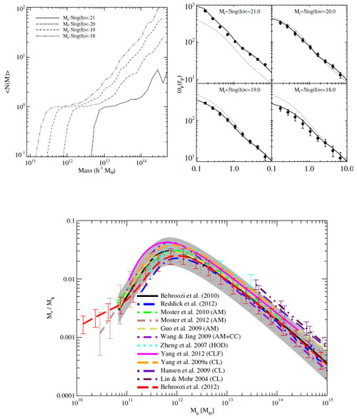 |
Figure 12. Illustration of HOD models of multiplicity functions (per halo) obtained from abundance matching (Conroy et al. 2006). Top right: Abundance matching prediction on the galaxy correlation function compared to SDSS observations (symbols), while the halo-halo correlation function is shown as dotted lines (Conroy et al. 2006). Bottom: Halo mass for given stellar mass obtained by abundance matching (AM), HOD, conditional luminosity function (CLF) and group catalogs (CL) at z = 0.1 (Behroozi et al. 2012). The shaded region shows the AM analysis of Behroozi et al. (2010). |
An offshoot of HOD models is to link the mean trend of some galaxy property in terms of the mass of its halo, using so-called Abundance Matching (AM). The idea is to solve N(> x) = N(> Mhalo), i.e. matching cumulative distributions of the observed galaxy property, x, with the predicted one for halo masses, determined either from theory (Press & Schechter 1974, Sheth et al. 2001) or from cosmological N body simulations (Warren et al. 2006, Tinker et al. 2008, Crocce et al. 2010, Courtin et al. 2011).
Common uses of AM involve one-to-one correspondences between 1) stellar and halo mass for central galaxies in halos, 2) total stellar mass and halo mass in halos, and 3) stellar and subhalo mass in galaxies. Marinoni & Hudson (2002) performed the first such AM analysis to determine Mhalo / L versus L; they first had to determine the observed cosmic stellar mass function, not counting the galaxies within groups, but only the groups themselves (Marinoni et al. 2002). Guo et al. (2010) used this third approach (called subhalo abundance matching or SHAM, and pioneered independently by Vale & Ostriker 2006 and Conroy et al. 2006), to determine the galaxy formation efficiency mstars / Mhalo as a function of Mhalo, by matching the observed stellar mass function with the subhalo mass function that they determined in the Millennium (Springel et al. 2005) and Millennium-II (Boylan-Kolchin et al. 2009) simulations. Although AM methods are based upon a fine relation between stellar and halo mass, they can easily be adapted to finite dispersion in this relation (Behroozi et al. 2010).
Not only is AM very useful to determine, without free parameters, the relation of stellar to halo mass (lower panel of Fig. 12), but it superbly predicts the galaxy correlation function of SDSS galaxies (Conroy et al. 2006, upper right panel of Fig. 12). The drawback of AM methods is that they do not clarify the underlying physics of galaxy formation.