


2.1. Counting the OB Stars: Harder than it Looks
Obviously most of the massive stars in a galaxy will be of O- and B-type simply because these are the spectroscopic types associated with the main-sequence, and stars spend ~ 90% of their lives on the main sequence. In addition, unlike the situation we will describe for yellow supergiants, and, to a lesser extent for red supergiants, there is little or none of the foreground contamination that makes it difficult to separate bona-fide extra-galactic O and B stars from foreground stars. Basically all blue stars in the field of a Local Group galaxy belong to that galaxy.
Yet, characterizing these massive stars is difficult. We need both the bolometric luminosity and effective temperature of a star to place it on the HRD; at the very least we need the bolometric luminosity to even guess the mass. And here we are hamstrung by physics: on the main-sequence these massive stars are so hot that the optical is way down on the tail of the Rayleigh-Jeans distribution. The problem is humorously sketched out in Figure 2 of Conti (1986).
Good photometry is essential to the process, and for that reason the
Local Group Galaxies Surveys (LGGS) was undertaken in the early 2000s,
designed to obtain UBVRI photometry to 1-2% or better for a
20 M star
(Massey et al. 2006,
2007a,
2007b).
This is complicated by the fact that O-type stars are by no means the
brightest stars in a galaxy. They are the most bolometrically luminous,
but they are several magnitudes fainter than, say, B or A supergiants of
much lesser mass. Typical V magnitudes for a
20M star
on the zero-age main-sequence (ZAMS)
run from 21.3 in M31, say, to 23.2 in IC 10, the latter due to its high
reddening; in contrast, such stars are found about 6 magnitudes brighter
in the LMC than in M31. The realm of the OB stars in the
color-magnitude
diagram of M31 is shown in Figure 2.
star
(Massey et al. 2006,
2007a,
2007b).
This is complicated by the fact that O-type stars are by no means the
brightest stars in a galaxy. They are the most bolometrically luminous,
but they are several magnitudes fainter than, say, B or A supergiants of
much lesser mass. Typical V magnitudes for a
20M star
on the zero-age main-sequence (ZAMS)
run from 21.3 in M31, say, to 23.2 in IC 10, the latter due to its high
reddening; in contrast, such stars are found about 6 magnitudes brighter
in the LMC than in M31. The realm of the OB stars in the
color-magnitude
diagram of M31 is shown in Figure 2.
 |
 |
Figure 2. Color-magnitude of M31. The upper diagram shows the observed data, while the lower one shows the expected contribution from foreground stars. From Drout et al. (2009) and used with permission. |
Such photometry allows us to determine the absolute visual magnitude if
the extinction is known, or if it can be estimated using
a combination of a reddening-free color index plus the observed colors
(see, e.g.,
Massey et al. 1989).
However, while necessary, photometry is not sufficient, not if we want
to know the approximate mass of the star. The reason is simple: the
conversion from absolute visual magnitude to bolometric magnitude is a
very steep function of the effective temperature, and the optical colors
are highly insensitive to the effective temperature.
Massey (1998a)
discusses this in detail, demonstrating that the Johnson Q
parameter changes by only 0.03 mag per 1 mag change in the bolometric
correction. This 1 mag change in the bolometric correction corresponds
to a change of 0.2 dex in the log of the mass, assuming a
mass-luminosity relationship of L ~ m2.0. In
other words, even the best optical photometry would lead to a
minimum uncertainty in the mass of 0.2 dex, the difference
(roughly) between a
30 M
star and a
50 M
star. In practice, 0.03 mag accuracy
in Q is very difficult to achieve (requiring 1% photometry in
both U-B and B-V),
and a more realistic error is probably 0.05 mag in Q,
corresponding to an uncertainty of 0.3 dex in the mass, or the
difference between a 30
M star
and one of 65
M.
Massey (1998a)
goes on to demonstrate that even near-UV colors
(such as using HST's F170 filter, centered at 1700 Å)
doesn't buy you more in terms of determining the effective temperature
from photometry.
However, spectroscopy answers this neatly. For O stars, the relative
strengths of He I and He II are very temperature dependent.
Modeling provides temperatures to about 1000 K or better, and at these
temperatures that corresponds to an uncertainty in the bolometric
correction of about 0.07 mag
2.
This translates to
an uncertainty of only 0.015 dex in the mass, the difference
between a 30
M star
and one of 31
M! Even
using spectral types to infer the
temperatures leads to a similar improvement; an uncertainty of a single
spectral type is a temperature difference of ~ 2000 K (see, e.g., Table
9 in
Massey et al. 2005b).
In the last few years, we've seen an explosion in our knowledge of the massive star contents of the nearby universe. The VLT-FLAMES survey of massive stars in the Magellanic Clouds (e.g., Evans et al. 2006, 2007; Mokiem et al. 2006, 2007) and the subsequent targeted study of the 30 Doradus region (e.g., Evans et al. 2011) have greatly improved our knowledge of the stellar content of our nearest extragalactic neighbors. These studies have not only produced spectral types, but also allowed detailed atmospheric analysis in many cases, e.g., Hunter et al. (2008).
One disadvantage of such studies is in regions of high surface
brightness nebulosity, such as the 30 Doradus region. With fiber
instruments (such as VLT-FLAMES) sky subtraction isn't local, unless
time is spent using small offsets. Nebula emission can contaminate the
critical He I triplet lines, e.g., He I
 4471. Our group has
started a program with Magellan to obtain high
signal-to-noise long-slit optical spectroscopy of the early-type stars
in NGC 346 and Lucke-Hodge 41. The former is the
brightest HII region in the SMC, while the latter is second in brightness and
richness only to 30 Doradus itself.
4471. Our group has
started a program with Magellan to obtain high
signal-to-noise long-slit optical spectroscopy of the early-type stars
in NGC 346 and Lucke-Hodge 41. The former is the
brightest HII region in the SMC, while the latter is second in brightness and
richness only to 30 Doradus itself.
A spectroscopic followup to the M31 and M33 LGGS requires large telescope aperture (given the faintness of the OB stars) and a multiplexing capability given the number of stars involved; this combination comes together in the 6.5-m MMT's Hectospec. Preliminary results for ~ 1700 stars were shown by Smart et al. (2012), and full results will be given by Massey et al. (2013). Of course, this too suffers from nebular contamination in regions of strong nebulosity, and in those cases we are planning long-slit spectroscopy.
Garcia et al. (2009, 2010), Herrero et al. (2012), and Garcia & Herrero (2013) have been doing similarly interesting work on the Local Group galaxy IC 1613, supplementing photometry with spectroscopy to study the young population. (IC 1613 was the only star-forming Local Group galaxy to be left out of the LGGS.) Their work has found a very interesting Of star that shows unexpected stellar wind characteristics among other discoveries (Herrero et al. 2012). Bresolin et al. (2007) has also discussed spectroscopy for ~ 50 early-type stars in IC 1613. Two O-type stars in WLM were discovered by Bresolin et al. (2006), along with ~ 25 B-type supergiants.
2.2. Luminous Blue Variables: Silent Quackers
Duncan (1922)
and
Hubble (1926)
first discovered several very bright, irregular variables in M33 and
M31, respectively. Among
these were Variable 1 in M33, and Variable 19 (AF And) in M31.
Hubble & Sandage
(1953)
used photographic plates of M31 and M33 dating from 1920 to 1953 in
order to study their properties, as well as to search for additional
examples. They found three
more in M33, which they designated Variables A, B, and C,
but no new ones in M31. They report on the characteristics of these
five stars,
noting that at their peaks they are among the brightest stars in these
galaxies (reaching a photographic blue magnitude of 15th),
and showing variability of the order of multiple magnitudes, except for
Var 19, where the amplitude was ~ 1 mag. In a footnote they likened
these "Hubble-Sandage variables" to that of S Doradus in the
LMC.
Eventually the connection to Galactic stars like
 Car and P
Cyg was made, and the term "Luminous Blue Variable," or LBV, was coined
by
Conti (1984).
Of the five original Hubble-Sandage variables, Variable A is usually no
longer listed as a "true" LBV since its spectrum developed TiO bands; see
Humphreys (1989).
At their most luminous, LBVs reach peak bolometric luminosities of about
106
L.
Car and P
Cyg was made, and the term "Luminous Blue Variable," or LBV, was coined
by
Conti (1984).
Of the five original Hubble-Sandage variables, Variable A is usually no
longer listed as a "true" LBV since its spectrum developed TiO bands; see
Humphreys (1989).
At their most luminous, LBVs reach peak bolometric luminosities of about
106
L.
Identifying a complete sample of LBVs in Local Group galaxies is probably not possible. Recall that most Galactic LBVs are known because they have happened to have outbursts during historical times. The last time the archetype LBV P Cygni did anything significant photometrically was in the 1600's. Massey (2006) has emphasized that if P Cyg were located in a nearby galaxy the star would not appear to be remarkable in any way unless we happened to take a spectrum of it.
Indeed, Massey (2006) happened upon such a star in M31. Its optical spectrum is indistinguishable from that of P Cyg; a comparison is shown in Figure 3. The helium and hydrogen lines show the characteristic P Cygni profiles, and even the NII lines are present, suggesting chemical enrichment of N at the surface.
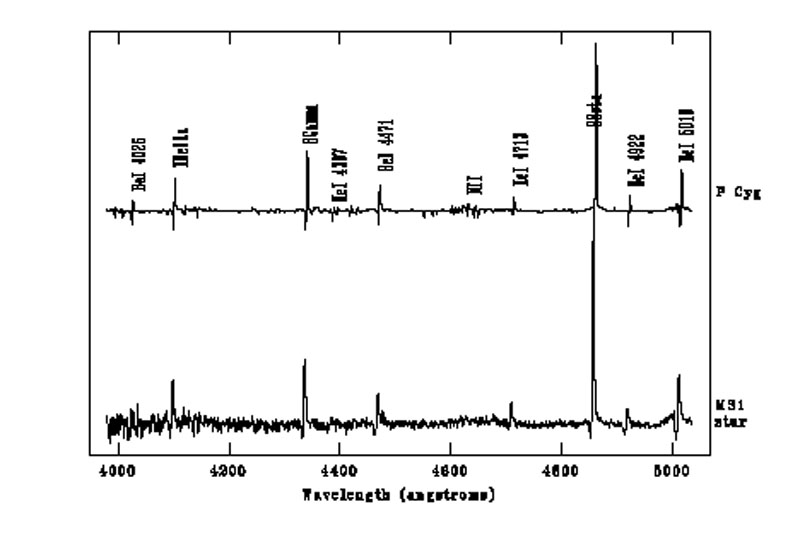 |
Figure 3. A comparison between the spectrum of P Cyg and the M31 star J004341.84+411112.0. From Massey (2006) and reproduced by permission. |
Massey et al. (2007a)
undertook a survey of H emission stars in the LGGS survey, finding many additional stars that
were spectroscopically identical to known LBVs. Are these stars true LBVs?
Bohannan (1997)
argued that
"A star should not be considered an LBV because its current
spectroscopic character is similar to that of a known LBV. Remember what
is said about ducks: it may look like a duck, walk like a duck, but it
is not a duck until it quacks." However, as
Massey et al. (2007a)
counter, "In a raft of ducks, at any one time, some will be quacking and
some will not. Momentary silence does not transform a duck into a goose,
nor would it confuse most bird spotters." One can further argue: if
these stars are not LBVs,
then what are they? In many cases their spectral signatures are unique.
emission stars in the LGGS survey, finding many additional stars that
were spectroscopically identical to known LBVs. Are these stars true LBVs?
Bohannan (1997)
argued that
"A star should not be considered an LBV because its current
spectroscopic character is similar to that of a known LBV. Remember what
is said about ducks: it may look like a duck, walk like a duck, but it
is not a duck until it quacks." However, as
Massey et al. (2007a)
counter, "In a raft of ducks, at any one time, some will be quacking and
some will not. Momentary silence does not transform a duck into a goose,
nor would it confuse most bird spotters." One can further argue: if
these stars are not LBVs,
then what are they? In many cases their spectral signatures are unique.
One way that could resolve the issue is to see whether there is evidence of past ejecta events, and such a study is currently underway using high spatial resolution HST spectroscopy in collaboration with Nathan Smith. Such studies should reveal if any of the LBV candidates in M31 and M33 have had past outbursts. Future photometric monitoring is also planned.
2.3. Yellow Supergiants: Looking at Stellar Evolution through a Magnifying Glass
As a massive star evolves to the red supergiant phase, it briefly
becomes a yellow supergiant. If the star also evolves back to the blue
(expected for stars of about 30
M), it will
again pass through a YSG phase. The length of this phase is measured not
in million of years, but rather in thousands of years, about 0.1% of the
star's lifetime. The brevity of this phase only adds to the usefulness
of studying these objects.
From a stellar evolutionary point of view, these stars act as "a sort of
a magnifying glass, revealing relentlessly the faults of calculations of
earlier phases," as
Kippenhahn & Weigert
(1994)
put it.
Still, to capitalize on this phase, we must first identify a relatively complete sample. The difficulty here is that there is a sea of foreground yellow dwarfs of the same color and magnitude range seen either against the Magellanic Clouds or the more distant members of the Local Group. For the red supergiants (discussed below in Section 2.4) we can separate foreground dwarfs from extragalactic stars by the use of two-color indices. But, no such photometric trick works for YSGs.
Instead, we must rely upon radial velocities to separate foreground contaminants from extragalactic YSGs. Fortunately, this works extremely well. In Figure 4 we show the observed radial velocities of yellow stars seen against the LMC, as found by Neugent et al. (2012b). The stars are all in the right magnitude and color range to be YSGs in the LMC. The vertical line at 278 km s-1 shows the average radial velocity of the LMC. The errors on the individual velocities are small (of order 1 km s-1); the dispersion about the systematic velocity of the LMC is due to that galaxy's rotation. Nevertheless, it's clear that a very clean separation exists between the low velocity foreground yellow dwarfs and the LMC's YSGs.
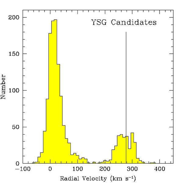 |
Figure 4. The radial velocities of YSG candidates seen against the LMC. The vertical line at 278 km s-1 shows the average radial velocity of the LMC. From Neugent et al. (2012b) and reproduced by permission. |
How significant is this contamination? For the LMC it's 80% (Neugent et al. 2012b); i.e., only 20% of the photometrically-chosen sample were found to be YSGs. For the SMC (Neugent et al. 2010) it was similar, about 65% were foreground. The situation was even worse for M31 (Drout et al. 2009), where the contamination reached 96%.
These studies have proven quite useful for evaluating the Geneva
evolutionary models.
Drout et al. (2009)
identified a sample of YSGs in M31 that was unbiased in
luminosity. Placing the stars on the HRD, they determined the relative
number in each mass bin, and compared this to the predictions of the
evolutionary models. The number expected in the 20-25
M bin,
compared to that in the 15-20
M mass
bin will just be proportional to the
relative lifetimes weighted by the initial mass function, assuming that
the average star formation rate within a galaxy hasn't changed
appreciably during the past few million years. What they found was
rather surprising. On the one hand, the evolutionary models did a good
job of predicting the locations of the YSGs in the HRD, in the sense
that they did not predict higher luminosity YSGs than those that were
observed. However, in terms of the relative lifetimes, the models
disagreed badly with the observation: there were far fewer high
luminosity YSGs than those predicted by the models.
Neugent et al. (2010)
extended this work to the SMC, with similar results. Since the SMC is
metal-poor, while M31 is metal-rich (see
Table 1), this eliminated
errors in the assumed mass-loss rates from the list of possible
explanations.
However, just as observational methods improve, so does theory. Drout et al. (2012) and Neugent et al. (2012b) extended these studies to M33 and the LMC. However, by that time, new versions of the Geneva evolutionary models had become available (e.g., Ekström et al. 2012) and both studies now found excellent agreement between the new models and the distribution of stars in the HRD. As Drout et al. (2012) argued, the better agreement could not be due to a single cause, but due to a combination of improvements. These include a better prescription for mass loss during the RSG phase, which affects the subsequent evolution from the red back to the blue side of the HRD. The new models also adopt a new shear diffusion coefficient, and more realistic initial rotation velocities. But, Drout et al. (2012) argue that even so, these changes by themselves could not explain the entire improvement. Instead, the improved initial compositions and opacities must be important factors as well. Regardless, while the older models did not do a good job predicting the relative numbers of YSGs as a function of luminosity, the newer models do an excellent job.
2.4. Red Supergiants: Big and Sometimes Too Cool
The subject of red supergiants has been recently reviewed in this journal by Levesque (2010) and elsewhere by Levesque (2012), and the interested reader can find out much more about these fascinating objects in those two reviews. Here we briefly summarize and complement these excellent papers.
Most massive stars spend the majority of their He-burning lives as red supergiants, and yet until relatively recently this phase was poorly studied. Massey & Olsen (2003) were the first to note a significant discrepancy between the locations of RSGs and the evolutionary tracks: if one used the standard spectral-type to effective temperature conversions, then RSGs were much cooler than evolutionary tracks predicted. Improved tracks became available, and yet the discrepency remained. Using the newly available atmospheric models, Levesque et al. (2005) determined a new effective temperature scale of Galactic stars, bringing into agreement for the first time the locations of RSGs in the HRD and the evolutionary tracks. We show the improvement in Figure 5.
 |
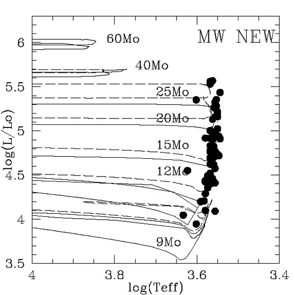 |
Figure 5. The effect of the new RSG effective temperature scale. On the left is shown the poor agreement between the "observed" location of RSGs in the HRD based on the old effective temperature scale and the evolutionary tracks. On the right is shown the improvement from Levesque et al. (2005). This figure is based upon one in Levesque et al. (2005) and Levesque (2010). |
|
Like the YSGs, identification of the RSGs among the galaxies of the Local Group is complicated by foreground contamination. This turns out not to be much of a problem for RSGs in the Magellanic Clouds, as shown by Neugent et al. (2012b), and shown here in Figure 6. (Compare this to Figure 4.) But that is just because the RSGs in the Magellanic Clouds are bright (V ~ 12-13; see Neugent et al. 2012b and Levesque et al. 2006), and any foreground red dwarfs would have to be within about 50 pc of the sun to be of similar brightness. The story is quite different for galaxies such as M31 and M33, where the typical RSG will be 6 mags fainter, and red foreground dwarfs will be at the right brightness at distances of 800 pc, meaning that the surface density of foreground objects will be 250× greater.
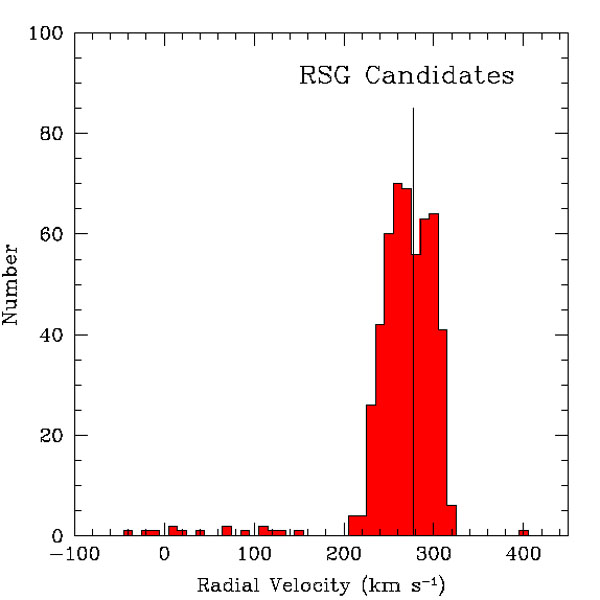 |
Figure 6. The radial velocities of RSG candidates seen against the LMC. The vertical line at 278 km s-1 shows the average radial velocity of the LMC. For the RSGs in the LMC, foreground contamination is minimal, unlike the case for the YSGs (compare to Figure 4). From Neugent et al. (2012b) and reproduced by permission. |
This problem is readily apparent if one compares the distribution of blue and red stars in M33; see, for example, Figures 21 and 22 of Humphreys & Sandage (1980). The blue stars are clumped, while the red stars show a far more uniform surface distribution. The explanation for this cannot be one of age, as pointed out by Massey (1998b); rather, it must be that foreground contamination dominates.
Massey (1998b) found that it was relatively easy to separate extragalactic RSGs from foreground dwarfs by means of a B-V vs V-R two-color diagram. At these low effective temperatures (< 4000 K) V-R is primarily a measure of effective temperature, while B-V is dominated by surface gravity effects due to line-blanketing. Such a diagram for red stars seen towards M31 is shown in Figure 7. The dense band of (black) points are the presumed foreground stars, while the stars with the higher B-V values (shown in red) are the RSG candidates. Radial velocities demonstrated that the red points followed the rotation curve of M31, as shown in Figure 8.
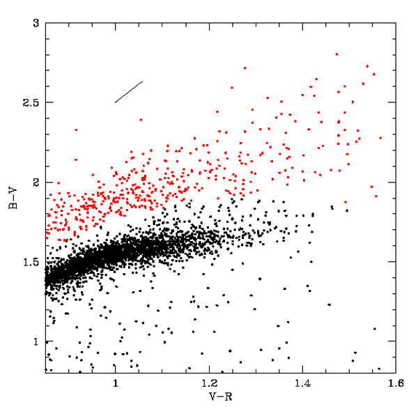 |
Figure 7. A two-color diagram of stars seen towards M31. There are two distributions in B-V, with the red points representing the (presumed) RSGs, and the black points representing the (presumed) foreground objects. The reddening vector is indicated by the line near the top; its size is roughly that of the reddening seen towards M31 stars. From Massey et al. (2009) and used with permission. |
 |
Figure 8. The radial velocities of the presumed RSGs (red points) from Figure 7 is shown superimposed on the rotation curve defined by the HII regions (crosses). The green points show the stars previously confirmed spectroscopically as RSGs by Massey (1998). From Massey et al. (2009) and used with permission. |
To date, the RSG content of the LMC is relatively well established (Neugent et al. 2012b), as is that of M31 (Massey et al. 2009), M33 (Drout et al. 2012), WLM and NGC 6822 (Levesque & Massey 2012). A comprehensive study of the RSG content of the SMC is still lacking, although Levesque et al. (2006) successfully modeled a number of previously known SMC RSGs, determining effective temperatures and reddenings.
One complication emphasized by Levesque (2010) is the potential confusion between RSGs and AGBs. Normal AGBs can be separated from RSGs by using a luminosity cut off (Brunish et al. 1986) as done by Massey & Olsen (2003). Recently a class of "super"-AGBs has been postulated and discussed (Siess 2006, 2007, Poelarends et al. 2008); these are stars in a narrow mass range that ignite carbon off-center. These stars could contaminate any sample of RSGs.
In general, our studies have shown that the coolest RSGs are warmer at low metallicities than at high metallicities; this is in agreement with the finding of Elias et al. (1985) that the average spectral type of RSGs is earliest in the SMC, a bit later in the LMC, and later still in the Milky Way, consistent with the progression in metallicity (see Table 1). This is a reflection of the shift in the Hayashi limit towards warmer temperatures with decreasing metallicity. The Hayashi limit represents the extreme effective temperature at which a star is still in hydrostatic equilibrium (Hayashi & Hoshi 1972). However, a startling discovery by Massey et al. (2007c) and Levesque et al. (2007) was that of a few of the most luminous RSGs and changed their spectral types quite significantly (e.g., K0 to M4) on the timescale of months. At the coolest these stars were much cooler than any of the other RSGs in their galaxies. These stars show large photometric variability, and changes in AV, consistent with episodic dust production. The nature of these objects is still unknown.
2.5. The Wolf-Rayet Stars: Easy to Find Some, but Tough to Find the Rest
Detecting complete samples of Wolf-Rayet stars sounds like it should be easy. After all, their spectra are marked by strong emission lines, and should be readily found either by objective prism surveys or by interference filter imaging 3. The problem, however, is that for a survey to be useful, it must be complete for both WCs and WNs if the relative ratios are going to be compared to that predicted by the evolutionary models.
Surveys are intrinsically flux-limited; i.e., they are sensitive
primarily to the emission line fluxes. Let us consider the line
strengths of
the strongest emission line in WC-type WRs,
C III 4650, vs that
of the strongest emission line in WN-type WRs,
He II 4686. The
difficulty is thus illustrated in Figure 9,
where we compare the equivalent widths (ews) of these strongest
lines. We have used the equivalent widths as a proxy for line flux; we
can do this (for the most part) as the absolute visual magnitudes are
quite similar between WC and (most) WN subtypes. The exception are the
WN7s, which are brighter (see, e.g., Table 3-2 in
Conti 1988).
The implications of this histogram is that WNs are harder
to find, and thus one must be demonstrate that one is complete to
sufficiently small line fluxes before claiming one has determined
the relative number of WC and WN stars.
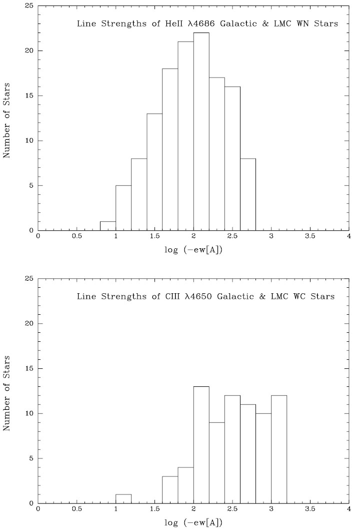 |
Figure 9. The equivalent widths (ew) of the strongest optical lines in WN and WC stars are compared. The data in this figure comes from Conti & Massey (1989), and the figure comes from Massey & Johnson (1998). Reproduced by permission. |
Early efforts to detect WRs in the nearby galaxies of the Local Group have been nicely summarized by Massey & Conti (1983), Massey & Johnson (1998), Neugent & Massey (2011) and Neugent et al. (2012a).
In the SMC, an objective prism survey by
Azzopardi & Breysacher
(1979a)
used an interference filter to isolate the strong
He II 4686 and/or
C III 4650 lines, and
found 4 new WRs, bringing the total at the time to 8, with the previous
4 found by general spectroscopic studies (see
Breysacher &
Westerlund 1978).
A ninth WR was found by
Morgan et al. (1991).
Massey & Duffy
(2001)
undertook an on-band, off-band interference filter
imaging campaign with a wide-area CCD camera. Photometry of 1.6 million
stellar images helped identify a number of candidates,
including all of the known SMC WRs, at high significance
levels. Follow-up spectroscopy then confirmed two new WNs, bringing the
total to 11, as well as a number of Of-type stars, demonstrating that
the survey was certainly sensitive enough to find even the weakest-lined
WNs. However, shortly following this spectroscopy we accidentally
discovered a 12th WR star in the SMC
(Massey et al. 2003).
This star had been too crowded to have been found in the
Massey & Duffy
(2001)
survey. Of these 12 WRs, 11 are of WN-type and only 1 is of
WC-type. This low WC/WN ratio is consistent with the SMC's low metallicity.
For the LMC, an objective prism survey by Azzopardi & Breysacher (1979b) discovered 11 new WRs to add to the already existing 80 that were known at the time (Fehrenbach et al. 1976), bringing the total to 91. The relatively small increase probably was due to the limited coverage in the Azzopardi & Breysacher (1979b) survey, with only a small fraction of the LMC surveyed. Since that time, many other WRs have been found, mostly by accidental spectroscopy. The latest catalog is that of Breysacher et al. (1999), which lists 134 WRs. Neugent et al. (2012c) discovered a rare WO star, and used the occasion to bring this list up to date by noting two stars that have been "demoted" to Of stars, and listing 6 other WRs since discovered by others. This brings the number known in the LMC to 139 stars, of which 107 are WN and 26 are WC or WO.
The early discovery of ~ 25 WRs in M33 by Wray & Corso (1972) really started the whole effort to discover WRs in Local Group galaxies beyond the Magellanic Clouds, and was responsible for the author's growing interest in graduate school in the subject of studying massive stars in nearby galaxies. Their work was followed by Conti & Massey (1981) and D'Odorico & Rosa (1981), who found numerous WRs in M33's HII regions. The first galaxy-wide systematic search (based on photographic on-band, off-band imaging) was described by Massey & Conti (1983), who presented spectral types and spectrophotometry for 79 WRs, about half of which had been previously known. Armandroff & Massey (1985) and Massey & Johnson (1998) provided CCD imaging in on- and off-band interference filters over a limited area to greatly improve the sensitivity and reveal mostly undiscovered WN-type WRs in M33. (At the time of Massey & Johnson (1998) the number of "spectroscopically confirmed" WRs in M33 had grown to 141, although as subsequently shown by Neugent & Massey 2011, a few of these were bogus, i.e., quasars or Of-type stars.) Finally, Neugent & Massey (2011) conducted an imaging survey that covered all of M33 using the Kitt Peak 4-m telescope and Mosaic CCD camera, with follow-up spectroscopy with the 6.5-m MMT and the 300-fiber spectrograph Hectospec. Their work found 55 new WRs, mostly of WN types, bringing the total known to 206, a number that they argue is complete to 5%.
Previous studies (e.g., Armandroff & Massey 1985, Massey & Johnson 1998, Massey & Duffy 2001) replied upon doing photometry of all the stellar images and then looking for magnitude differences from the on-band to the continuum that were statistically significant. This was not only time-consuming, but often failed because in some cases groups of stars would be photometered as 7 stars on one image but 6 on another: crowding matters. It also tended produce a lot of false positives: Neugent & Massey (2011) instead built on the image-subtraction techniques that had been developed over the years primarily to identify supernovae. An example of how the technique works is shown in Figure 10.
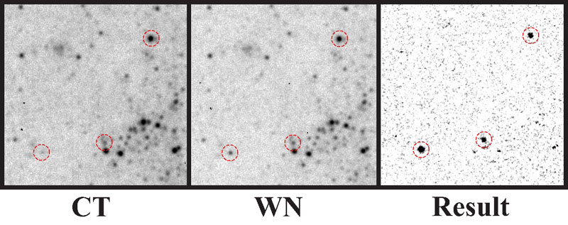 |
Figure 10. The power of the image subtraction technique is shown. The figure on the left is the off-band continuum ("CT") image, the middle image is the on-band WR image ("WN"), and the difference image is shown on the right ("Result"). From Neugent & Massey (2011) and reproduced by permission. |
One of the very attractive things about studying the WR content of M33
has always been the expectation that it has a metallicity
gradient. Would this be reflected in the relative population of WC and
WN? Even in the 1970s it was known that the SMC contained predominantly
WNs while the LMC contained a better mixture of WC and WNs, and
this was attributed to the fact the SMC had lower metallicity than the
LMC. Figure 11 shows the
results from
Neugent & Massey
(2011)'s
large sample, where
 is the galactocentric distance within the
plane of M33. The distribution of M33's WRs in shown in
Figure 12.
is the galactocentric distance within the
plane of M33. The distribution of M33's WRs in shown in
Figure 12.
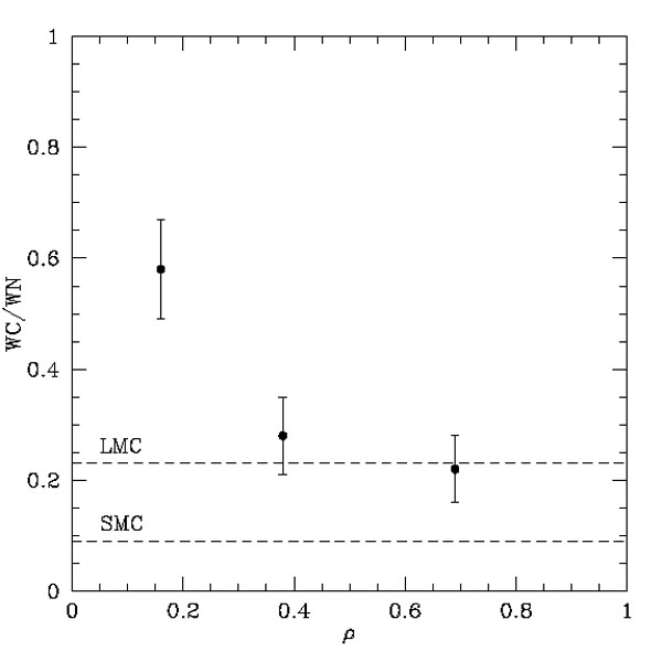 |
Figure 11. M33 WC/WN ratio vs
galactocentric distance. The ratio of the number of WC-type and WN-type
WRs is plotted against the galactocentric distance ρ within the
plane of M33. A value of
|
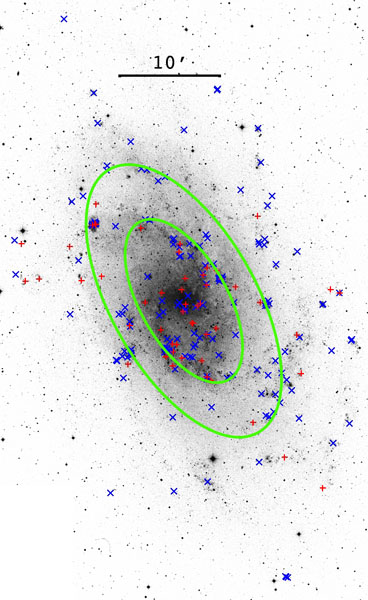 |
Figure 12. The distribution of WRs in
M33. The red +'s represent the WC-type WRs while the
blue x's represent
the WN-type WRs. The two green ovals represent galactocentric distances
of |
In terms of WR surveys, M31 has proven a very hard nut to crack, due to the galaxy's very large angular size. At the same time, M31 is perhaps the most interesting, as its metallicity is about two times solar (Zaritsky et al. 1994, Sanders et al. 2012; see discussion in Neugent et al. 2012a), providing a key test of stellar evolutionary models. Until recently, only photographic surveys had been carried out galaxy-wide (Moffat & Shara 1983, 1987), finding mostly WCs, presumably due to poor sensitivity. Massey et al. (1986) used much deeper CCD imaging on a few selected OB associations, finding a better mixture of WNs and WCs. The total number of WRs known by the time of the analysis of Massey & Johnson (1998) was 48, which gave a WC to WN ratio of 2.2. Massey & Johnson (1998) argued that if the sample was just restricted to the regions that were complete, the WC to WN ratio would likely be much lower, about 0.93. Nevertheless this was much higher than the evolutionary models predicted (Meynet & Maeder 2005). Neugent et al. (2012a) surveyed the entire galaxy, similar to the study of M33, bringing the total number of known WRs to 154, and yielding a WC to WN ratio of 0.67. This is still higher than the older Geneva models predict (i.e., Meynet & Maeder 2005) but may be consistent with newer models once they become available at high metallicity. (See Figure 13.)
 |
Figure 13. The WC to WN ratio plotted against the oxygen abundance, which corresponds to 8.7 at z = 0.014 (solar). The red error bars indicate the measured uncertainties in the WC/WN ratio, while the black error bars show the √N uncertainties, which are more appropriate for comparing with the evolutionary model. The two blue lines show the prediction for the new Geneva models (the upper one being with no rotation, and the lower one being with an initial rotation of 40% of the break up speed), while the dashed line shows the prediction from the older Geneva models. From Neugent et al. (2012a), and reproduced by permission. |
What about the irregular dwarfs beyond the Magellanic Clouds? Westerlund et al. (1983) used a "grism" to detect one WR (WN-type) star in NGC 6822; Armandroff & Massey (1985) sampled most of this galaxy searching for WRs, and detected three other WNs that were eventually confirmed by spectroscopy (Massey et al. 1987). A WO-type WR is known in IC 1613; it was discovered by D'Odorico & Rosa (1982) as part of a survey of the ionizing stars of H II regions, and subsequently studied by Davidson & Kinman (1982) and others (see, e.g., Massey et al. 1987, Kingsburgh & Barlow 1995). No additional WRs have been found.
The case of IC 10 deserves a special note. Massey et al. (1992) found 22 WR candidates, of which 15 were confirmed by spectroscopy. This was a spectacularly large number, given that IC 10 is about half of the size of the SMC (van den Bergh 2000), and led to the galaxy's recognition as a starburst. We now understand that the burst is being triggered by infalling gas from an extended cloud that is counter-rotating with respect to the galaxy itself, as shown by Wilcots & Miller (1998). Of the 15 spectroscopically confirmed IC 10 WRs listed by Massey & Johnson (1998), 10 are of WC type, making the WC/WN ratio at that time be 2. This was absurdly high given IC 10's relative poor metallicity (log O/H + 12 = 8.2; see Table 1). Even in the LMC, where log O/H + 12 = 8.4 the WC to WN ratio is 0.24, a factor of 8 lower. This stood as a mystery until a much more sensitive survey was conducted by Massey & Holmes (2002). This survey suggested that the total number of WR stars in IC 10 is even more remarkable than previously thought, of order 100. If so, this could bring the WC to WN ratio down to 0.3, about as expected, but would require a surface density of WRs that is 20× greater than that of the LMC. Only two of the new WR candidates had been confirmed by Massey & Holmes (2002) though. Further follow-up is planned this coming year when Binospec is implemented on the MMT.
Beyond the Local Group, surveys for WRs have been conducted in NGC 300 (Schild & Testor 1991, 1992; Breysacher et al. 1997; Schild et al. 2003), M83 (Hadfield et al. 2005), NGC 1313 (Hadfield & Crowther 2007), NGC 7793 (Bibby & Crowther 2010), NGC 5068 (Bibby & Crowther 2012), and M101 (Shara et al. 2013) among others. The problem is, of course, that these galaxies are found at distances ranging from 2.0 Mpc (NGC 300) to 7.0 Mpc (M83, M101), compared to, say, the distance to M33 (0.8 Mpc). So, the stars are going to be 1.9-4.6 mag fainter, and crowding (although getting to be an issue in M33; see Neugent & Massey 2011) a factor of 2.4-8.4× worse. It would seem very difficult to identify an unbiased (much less complete) population of WRs in these galaxies if the goal is to compare relative populations.
2 For O stars, the bolometric correction goes as roughly -6.90 logTeff +27.99, so a change of 1,000 K at 40,000 K corresponds to 0.07 mag. Back.
3 An unconfirmed rumor has it that one Time Allocation Committee wag, debating one of the author's proposal for Kitt Peak 4-meter time to search for WRs in M31, claimed that he could find these using a 12-inch telescope in his backyard. Back.