

Rapid advances in observational cosmology have led to the establishment of a precision cosmological model, with many of the key cosmological parameters determined to one or two significant figure accuracy. Particularly prominent are measurements of cosmic microwave background (CMB) anisotropies, with the highest precision observations being those of the Planck Satellite [1, 2] which for temperature anisotropies supersede the iconic WMAP results [3, 4]. However the most accurate model of the Universe requires consideration of a range of different types of observation, with complementary probes providing consistency checks, lifting parameter degeneracies, and enabling the strongest constraints to be placed.
The term `cosmological parameters' is forever increasing in its scope, and nowadays often includes the parameterization of some functions, as well as simple numbers describing properties of the Universe. The original usage referred to the parameters describing the global dynamics of the Universe, such as its expansion rate and curvature. Also now of great interest is how the matter budget of the Universe is built up from its constituents: baryons, photons, neutrinos, dark matter, and dark energy. We need to describe the nature of perturbations in the Universe, through global statistical descriptors such as the matter and radiation power spectra. There may also be parameters describing the physical state of the Universe, such as the ionization fraction as a function of time during the era since recombination. Typical comparisons of cosmological models with observational data now feature between five and ten parameters.
1.1. The global description of the Universe
Ordinarily, the Universe is taken to be a perturbed Robertson-Walker
space-time with dynamics governed by Einstein's equations. This is
described in detail by Olive and Peacock in this volume.
Using the density parameters
 i for the
various matter species and
i for the
various matter species and
 for
the cosmological constant, the Friedmann equation can be written
for
the cosmological constant, the Friedmann equation can be written
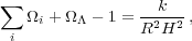 |
(1) |
where the sum is over all the different species of material in the
Universe. This equation applies at any epoch, but later in this
article we will use the symbols
i and
to
refer to the present values.
The complete present state of the homogeneous Universe can be
described by giving the current values of all the density parameters
and the Hubble constant h (the present-day Hubble parameter being
written H0 = 100 h km s-1
Mpc-1). A typical collection would be baryons
b,
photons  ,
neutrinos
,
neutrinos  , and cold dark matter
c (given
charge neutrality, the
electron density is guaranteed to be too small to be worth considering
separately and is included with the baryons). The spatial curvature can
then be determined from the other parameters using
Equation (1). The total present matter density
m
= c +
b is
sometimes used in place of the cold dark matter density
c.
, and cold dark matter
c (given
charge neutrality, the
electron density is guaranteed to be too small to be worth considering
separately and is included with the baryons). The spatial curvature can
then be determined from the other parameters using
Equation (1). The total present matter density
m
= c +
b is
sometimes used in place of the cold dark matter density
c.
These parameters also allow us to track the history of the Universe back in time, at least until an epoch where interactions allow interchanges between the densities of the different species, which is believed to have last happened at neutrino decoupling, shortly before Big Bang Nucleosynthesis (BBN). To probe further back into the Universe's history requires assumptions about particle interactions, and perhaps about the nature of physical laws themselves.
The standard neutrino sector has three flavors. For neutrinos of mass in the range 5 × 10⁻⁴ eV to 1 MeV, the density parameter in neutrinos is predicted to be
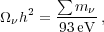 |
(2) |
where the sum is over all families with mass in that range (higher masses need a more sophisticated calculation). We use units with c = 1 throughout. Results on atmospheric and Solar neutrino oscillations [5] imply non-zero mass-squared differences between the three neutrino flavors. These oscillation experiments cannot tell us the absolute neutrino masses, but within the simple assumption of a mass hierarchy suggest a lower limit of approximately 0.06 eV on the sum of the neutrino masses.
Even a mass this small has a potentially observable effect on the formation of structure, as neutrino free-streaming damps the growth of perturbations. Analyses commonly now either assume a neutrino mass sum fixed at this lower limit, or allow the neutrino mass sum as a variable parameter. To date there is no decisive evidence of any effects from either neutrino masses or an otherwise non-standard neutrino sector, and observations impose quite stringent limits, which we summarize in Section 3.4. However, we note that the inclusion of the neutrino mass sum as a free parameter can affect the derived values of other cosmological parameters.
1.2. Inflation and perturbations
A complete model of the Universe should include a description of deviations from homogeneity, at least in a statistical way. Indeed, some of the most powerful probes of the parameters described above come from the evolution of perturbations, so their study is naturally intertwined in the determination of cosmological parameters.
There are many different notations used to describe the perturbations,
both in terms of the quantity used to describe the perturbations and
the definition of the statistical measure. We use the dimensionless
power spectrum
 2 as
defined in Olive and Peacock (also
denoted
2 as
defined in Olive and Peacock (also
denoted  in some of the
literature). If the perturbations
obey Gaussian statistics, the power spectrum provides a complete
description of their properties.
in some of the
literature). If the perturbations
obey Gaussian statistics, the power spectrum provides a complete
description of their properties.
From a theoretical perspective, a useful quantity to describe the
perturbations is the curvature perturbation
 , which measures
the spatial curvature of a comoving slicing of the space-time. A simple case
is the Harrison-Zel'dovich spectrum, which corresponds to a constant
2. More
generally, one
can approximate the spectrum by a power-law, writing
, which measures
the spatial curvature of a comoving slicing of the space-time. A simple case
is the Harrison-Zel'dovich spectrum, which corresponds to a constant
2. More
generally, one
can approximate the spectrum by a power-law, writing
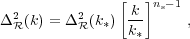 |
(3) |
where ns is known as the spectral index, always defined so that ns = 1 for the Harrison-Zel'dovich spectrum, and k* is an arbitrarily chosen scale. The initial spectrum, defined at some early epoch of the Universe's history, is usually taken to have a simple form such as this power-law, and we will see that observations require ns close to one. Subsequent evolution will modify the spectrum from its initial form.
The simplest mechanism for generating the observed
perturbations is the inflationary cosmology, which posits a period of
accelerated expansion in the Universe's early stages
[7,
8].
It is a useful working hypothesis that
this is the sole mechanism for generating perturbations, and it may
further be assumed to be the simplest class of inflationary model,
where the dynamics are equivalent to that of a single scalar field
 with
canonical kinetic energy slowly rolling on a potential
V().
One may seek to verify that this simple picture can match observations
and to determine the properties of
V()
from the observational data. Alternatively,
more complicated models, perhaps motivated by contemporary fundamental
physics ideas, may be tested on a model-by-model basis.
with
canonical kinetic energy slowly rolling on a potential
V().
One may seek to verify that this simple picture can match observations
and to determine the properties of
V()
from the observational data. Alternatively,
more complicated models, perhaps motivated by contemporary fundamental
physics ideas, may be tested on a model-by-model basis.
Inflation generates perturbations through the amplification of quantum fluctuations, which are stretched to astrophysical scales by the rapid expansion. The simplest models generate two types, density perturbations which come from fluctuations in the scalar field and its corresponding scalar metric perturbation, and gravitational waves which are tensor metric fluctuations. The former experience gravitational instability and lead to structure formation, while the latter can influence the CMB anisotropies. Defining slow-roll parameters, with primes indicating derivatives with respect to the scalar field, as
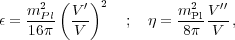 |
(4) |
which should satisfy  ,
|
,
| |
≪ 1, the spectra can be
computed using the slow-roll approximation as
|
≪ 1, the spectra can be
computed using the slow-roll approximation as
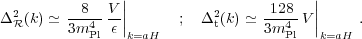 |
(5) |
In each case, the expressions on the right-hand side are to be evaluated when the scale k is equal to the Hubble radius during inflation. The symbol `≃' here indicates use of the slow-roll approximation, which is expected to be accurate to a few percent or better.
From these expressions, we can compute the spectral indices [9]
 |
(6) |
Another useful quantity is the ratio of the two spectra, defined by
 |
(7) |
We have
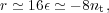 |
(8) |
which is known as the consistency equation.
One could consider corrections to the power-law
approximation, which we discuss later. However, for now we make the
working assumption that the spectra can be approximated by power
laws. The consistency equation shows that r and
nt are
not independent parameters, and so the simplest inflation models give
initial conditions described by three parameters, usually taken as
2, ns, and r, all to
be evaluated at some scale
k*, usually the `statistical center' of the
range explored by the
data. Alternatively, one could use the parametrization V,
, and
, all
evaluated at a point on the putative inflationary potential.
After the perturbations are created in the early Universe, they undergo a complex evolution up until the time they are observed in the present Universe. While the perturbations are small, this can be accurately followed using a linear theory numerical code such as CAMB or CLASS [10]. This works right up to the present for the CMB, but for density perturbations on small scales non-linear evolution is important and can be addressed by a variety of semi-analytical and numerical techniques. However the analysis is made, the outcome of the evolution is in principle determined by the cosmological model, and by the parameters describing the initial perturbations, and hence can be used to determine them.
Of particular interest are CMB anisotropies. Both the total intensity and two independent polarization modes are predicted to have anisotropies. These can be described by the radiation angular power spectra Cℓ as defined in the article of Scott and Smoot in this volume, and again provide a complete description if the density perturbations are Gaussian.
1.3. The standard cosmological model
We now have most of the ingredients in place to describe the
cosmological model. Beyond those of the previous subsections,
we need a measure of the ionization
state of the Universe. The Universe is
known to be highly ionized at low redshifts (otherwise radiation from
distant quasars would be heavily absorbed in the ultra-violet), and
the ionized electrons can scatter microwave photons altering the
pattern of observed anisotropies. The most convenient parameter to
describe this is the optical depth to scattering
 (i.e., the
probability that a given photon scatters once); in the approximation
of instantaneous and complete reionization, this could equivalently
be described by the redshift of reionization zion.
(i.e., the
probability that a given photon scatters once); in the approximation
of instantaneous and complete reionization, this could equivalently
be described by the redshift of reionization zion.
As described in comb, models based on these parameters
are able to give a good fit to the complete set of high-quality data
available at present, and indeed some simplification is
possible. Observations are consistent with spatial flatness, and
indeed the inflation models so far described automatically generate
negligible spatial curvature, so we can set k = 0; the density
parameters then must sum to unity, and so one can be eliminated. The
neutrino energy density is often not taken as an independent
parameter. Provided the neutrino sector has the standard interactions,
the neutrino energy density, while relativistic, can be related to the
photon density using thermal physics arguments, and a minimal assumption
takes the neutrino mass sum to be that of the lowest mass solution to
the neutrino oscillation constraints, namely 0.06 eV. In
addition, there is no observational evidence for the existence of
tensor perturbations (though the upper limits are fairly weak), and so
r could be set to zero. This leaves seven
parameters, which is the smallest set that can usefully be compared to
the present cosmological data set. This model is referred to by various
names, including
CDM, the
concordance cosmology, and the standard cosmological model.
Of these parameters, only
r is
accurately measured directly. The radiation density is dominated by the
energy in the CMB, and the COBE satellite FIRAS experiment determined its
temperature to be T = 2.7255 ± 0.0006 K
[12],
1
Unless stated otherwise, all quoted uncertainties in this article are
one-sigma/68% confidence and all upper limits are 95% confidence.
Cosmological parameters sometimes have significantly non-Gaussian
uncertainties. Throughout we have rounded central values, and
especially uncertainties, from original sources in cases where they
appear to be given to excessive precision. corresponding to
r =
2.47 × 10⁻⁵ h-2. It
typically need not be varied in fitting other data. Hence the minimum
number of cosmological parameters varied in fits to data is six, though
as described below there may additionally be many `nuisance' parameters
necessary to describe astrophysical processes influencing the data.
In addition to this minimal set, there is a range of other parameters which might prove important in future as the data-sets further improve, but for which there is so far no direct evidence, allowing them to be set to a specific value for now. We discuss various speculative options in the next section. For completeness at this point, we mention one other interesting parameter, the helium fraction, which is a non-zero parameter that can affect the CMB anisotropies at a subtle level. Fields, Molaro and Sarkar in this volume discuss current measures of this parameter. It is usually fixed in microwave anisotropy studies, but the data are approaching a level where allowing its variation may become mandatory.
Most attention to date has been on parameter estimation, where a set of parameters is chosen by hand and the aim is to constrain them. Interest has been growing towards the higher-level inference problem of model selection, which compares different choices of parameter sets. Bayesian inference offers an attractive framework for cosmological model selection, setting a tension between model predictiveness and ability to fit the data.
The parameter list of the previous subsection is sufficient to give a
complete description of cosmological models which agree with
observational data. However, it is not a unique parameterization, and
one could instead use parameters derived from that basic
set. Parameters which can be obtained from the set given above include
the age of the Universe, the present horizon distance, the present
neutrino background temperature, the epoch of matter-radiation
equality, the epochs of recombination and decoupling, the epoch of
transition to an accelerating Universe, the baryon-to-photon ratio,
and the baryon to dark matter density ratio. In addition, the
physical densities of the matter components,
i
h2, are often
more useful than the density parameters. The density perturbation
amplitude can be specified in many different ways other than the
large-scale primordial amplitude, for instance, in terms of its effect
on the CMB, or by specifying a short-scale quantity, a common choice
being the present linear-theory mass dispersion on a scale of 8
h-1 Mpc, known as
 8.
8.
Different types of observation are sensitive to different subsets of the full cosmological parameter set, and some are more naturally interpreted in terms of some of the derived parameters of this subsection than on the original base parameter set. In particular, most types of observation feature degeneracies whereby they are unable to separate the effects of simultaneously varying several of the base parameters.
1 Unless stated otherwise, all quoted uncertainties in this article are one-sigma/68% confidence and all upper limits are 95% confidence. Cosmological parameters sometimes have significantly non-Gaussian uncertainties. Throughout we have rounded central values, and especially uncertainties, from original sources in cases where they appear to be given to excessive precision. Back.