7. ALTERNATIVE METHODS

In Sections 3-6, we have reviewed in detail the four observational methods that have been most widely discussed, and applied, as probes for the origin of cosmic acceleration. We now review more briefly some of the other techniques for testing cosmic acceleration models. In some cases, surveys conducted for SN, BAO, or WL studies will automatically provide the data needed for these alternative methods. For example, redshift-space distortions (Section 7.2) and the Alcock-Paczynksi effect (Section 7.3) can be measured in galaxy redshift surveys designed for BAO measurements, and synoptic surveys designed for Type Ia supernovae will discover other transients that might provide alternative distance indicators (Section 7.4). Just as cluster investigations will increase the cosmological return from WL surveys, these methods will increase the return from BAO or SN surveys. The potential gains are large, but they are uncertain because the level of theoretical or observational systematics for these methods has not yet been comprehensively explored. In Section 8.5 we will examine how precisely our fiducial Stage III or Stage IV CMB+SN+BAO+WL programs predict the observables of these methods, setting targets for the precision and accuracy they should achieve to make major contributions to cosmic acceleration studies.

Some of the other methods described below require completely different types of observations or experiments, falling outside of the "survey mode" that characterizes the methods we have discussed so far. Compared to the combined SN+BAO+WL+CL approach, these methods may yield more limited information or be sensitive only to certain classes of acceleration models, but they can provide high-precision tests of the standard ΛCDM model, and they could yield surprising results that would give strong guidance to the physical origin of acceleration.

7.1. Measurement of the Hubble Constant at z ≈ 0

As emphasized by Hu (2005), a precise measurement of the Hubble constant, when combined with CMB data, allows a powerful test of dark energy models and tightened constraints on cosmological parameters. In effect, the CMB and H₀ provide the longest achievable lever arm for measuring the evolution of the cosmic energy density, from z ≈ 1100 to z = 0. The sensitivity of H₀ to dark energy is illustrated in Figure 2, which shows that a change Δw = ± 0.1 alters the predicted value of H₀ by 5% in Ω_k=0 models that are normalized to produce the same CMB anisotropies. More generally, a low redshift determination of the Hubble constant combined with Planck-level CMB data constrains w with an uncertainty that is twice the fractional uncertainty in H₀, assuming constant w and flatness. The challenge for future H₀ studies is to achieve the percent-level statistical and systematic uncertainties needed to remain competitive with other cosmic acceleration methods. Freedman and Madore (2010) review recent progress in H₀ determinations and prospects for future improvements; the past five years have seen substantial advances in both statistical precision and reduction of systematic uncertainties.

One of the defining goals of the Hubble Space Telescope was to measure H₀ to an accuracy of 10%. The H₀ Key Project achieved this goal, with a final estimate H₀ = 72 ± 8 km s^-1 Mpc^-1 (Freedman et al. 2001), where the error bar was intended to encompass both statistical and systematic contributions. This estimate used Cepheid-based distances to relatively nearby (D < 25 Mpc) galaxies observed with WFPC2 to calibrate a variety of secondary distance indicators — Type Ia supernovae, Type II supernovae, the Tully-Fisher relation of disk galaxies, and the fundamental plane and surface-brightness fluctuations of early-type galaxies. These secondary indicators were in turn applied to galaxies "in the Hubble flow," meaning galaxies at large enough distance (D ≈ 40-400 Mpc) that their peculiar velocities v_pec did not contribute significant uncertainty when computing H₀ = v / d. The Cepheid period-luminosity (P-L) relation was calibrated to an adopted distance modulus of 18.50 ± 0.10 mag for the Large Magellanic Cloud (LMC). The uncertainty in adjusting the LMC optical P-L relation to the higher characteristic metallicities of calibrator galaxies was an important contributor to the final error budget; Freedman et al. (2001) adopted a ± 0.2 mag/dex uncertainty in the metallicity dependence, implying a ~ 0.07 mag systematic uncertainty in the correction (3.5% in distance). Another important systematic was the uncertainty in differential measurements of Cepheid fluxes and colors over a wide dynamic range along the distance ladder. The uncertainty of the LMC distance itself was also a significant fraction of the error budget.

A number of subsequent developments have allowed substantial improvements in the measurement of H₀ (see Riess et al. 2009, Riess et al. 2011, Freedman and Madore 2010, Freedman et al. 2012). The recent determination of H₀ = 73.8 ± 2.4 km s^-1 Mpc^-1 by Riess et al. (2011) yields a 1σ uncertainty of only 3.3%, including all identified sources of systematic uncertainty and calibration error. One important change in this analysis is a shift to Cepheid calibration based on the maser distances to NGC 4258 (Herrnstein et al. 1999, Humphreys et al. 2008, Humphreys et al. 2013) and on parallaxes to Galactic Cepheids measured with Hipparcos (van Leeuwen et al. 2007) and with the HST fine-guidance sensors (Benedict et al. 2007). These calibrations circumvent the statistical and systematic uncertainties in the LMC distance, and they directly calibrate the P-L relation in the metallicity range typical of calibrator galaxies, albeit with a sample of only ~ 10 stars reaching an error-on-the-mean of 2.8% in the case of Milky Way parallaxes. A second improvement is more than doubling the sample of "ideal" Type Ia SNe — with modern photometry, low-reddening, typical properties, and caught before maximum — from the two available to Freedman et al. (2001) to eight. Of all secondary distance indicators, Type Ia supernovae have the smallest statistical errors, and probably the smallest systematic errors, and they can be tied to large samples of supernovae observed at distances that are clearly in the Hubble flow. Riess et al. (2009, 2011) use Type Ia supernovae exclusively in their H₀ estimates. Third, Cepheid observations at near-IR wavelengths (1.6μm) have reduced uncertainties associated with extinction and the dependence of Cepheid luminosity on metallicity (Riess et al. 2012). Finally, relative calibration uncertainties of Cepheid photometry obtained with different instruments and photometric systems along the distance ladder have been mitigated by the use of a single instrument, HST's WFC3, for a large fraction of the data.

Extending the trend towards longer wavelength calibration, Freedman et al. (2011) and Scowcroft et al. (2011) argue that 3.6μm measurements — possible with Spitzer and eventually with JWST — minimize systematic uncertainties in the Cepheid distance scale because of low reddening and weak metallicity dependence. Monson et al. (2012) calibrate the 3.6μm P-L zero-point against Galactic Cepheid samples, including the Benedict et al. (2007) parallax sample, and thereby infer the distance modulus to the LMC as a test of the optical Cepheid P-L relation and its metallicity correction. Freedman et al. (2012) use these Milky Way parallaxes to calibrate the optical Cepheid P-L relation and then recalibrate the Key Project data set to infer H₀; this determination still relies on optical, WFPC2 Cepheid data (and the associated metallicity corrections and flux and color zero-point uncertainties), and the Key Project SN Ia calibrator sample includes several SNe with photographic photometry or high extinction. Sorce et al. (2012) use the Tully-Fisher (1977) relation in the Spitzer 3.6μm band, normalized to the Monson et al. (2012) LMC distance, to recalibrate the SN Ia absolute magnitude scale and thereby infer H₀. Suyu et al. (2012a) infer H₀ from gravitational lens time delays for two well constrained systems, an approach that sidesteps the traditional distance ladder entirely (see Section 7.10 for further discussion). These four recent H₀ determinations (Riess et al. 2011, Freedman et al. 2012, Sorce et al. 2012, Suyu et al. 2012a) agree with each other to better than 2%. While the data used for the first three are only partly independent, this level of consistency is nonetheless an encouraging indicator of the maturity of the field. With the precision of H₀ measurements already at a level that allows critical tests of dark energy models in combination with CMB, BAO, and SN data (see, e.g., Anderson et al. 2012), a key challenge for the field is convergence on error budgets that neither underrepresent the power of the data nor understate systematic uncertainties.

Over the next decade, it should be possible to reduce the uncertainty in direct measurement of H₀ to approach the one-percent level. One crucial step will be the 1% to 5% parallax calibration of hundreds of long-period Galactic Cepheids within 5 kpc by the Gaia mission, setting the fundamental calibration of the multi-wavelength P-L relation and, to some degree, its metallicity dependence on a solid geometrical base with distance precision easily better than 1%. New Milky Way parallax measurements using the spatial scanning capability of HST may achieve this precision even sooner. Discovery of additional galaxies with maser distances (like NGC 4258) may also improve the Cepheid calibration or, if they are in the Hubble flow, may provide a direct determination of the Hubble constant (see Reid et al. 2012a for a recent measurement of UGC 3789 and Greenhill et al. 2009 for additional candidates). The other key step will be the Cepheid calibration of more Type Ia supernovae, which occur at a rate of one per 2-3 years in the range D < 35 Mpc accessible to HST with WFC3. JWST could increase this range to D < 60 Mpc, quadrupling the rate of usable supernovae. Ultimately a sample of 20 to 30 calibrations of the SN Ia luminosity is needed to reduce the sample size contribution to uncertainty in H₀ below 1%. With firmer P-L calibration and a larger Type Ia sample, the remaining uncertainty in H₀ is likely to be dominated by systematic uncertainty in the linearity of the photometric systems observing nearby and distant Cepheids. This may be minimized by the careful construction of "flux ladders," analogous to distance ladders but used to compare the measurements of disparate flux levels. Additional contributions to the determination of H₀ with few percent precision could come from "golden" lensing systems, infrared Tully-Fisher distances, surface brightness fluctuation measurements further into the Hubble flow, Sunyaev-Zel'dovich effect measurements, and local volume measurements of BAO.

We discuss the potential contribution of H₀ measurements to dark energy constraints in Sections 8.3 and 8.5 below. Already, the combination of the 3% measurement of Riess et al. (2011) with CMB data alone yields w = -1.08 ± 0.10, assuming a flat universe with constant w. The limitation of H₀ is, of course, that it is a single number at a single redshift, so while it can test any well specified dark energy model, it provides little guidance on how to interpret deviations from model predictions. However, precision H₀ measurements can significantly increase the constraining power of other measurements: for our fiducial Stage IV program described in Section 8, assuming a w₀ - w_a model for dark energy, a 1% H₀ measurement would raise the DETF Figure of Merit by 40%. A direct measurement of H₀ also has the potential to reveal departures from the smooth evolution of dark energy enforced by the w₀ - w_a parameterization. In essence, the dark energy model transfers the absolute distance calibration from moderate redshift BAO measurements down to z = 0, but unusual low redshift evolution of dark energy can break this link, shifting H₀ away from its expected value. A precise determination of H₀, coupled to a w(z) parameterization that allows low-redshift variation, could reveal recent evolution of dark energy and definitively answer the basic question, "Is the universe still accelerating?"

7.2. Redshift-Space Distortions

As discussed in Section 2.3, peculiar velocities make large scale galaxy clustering anisotropic in redshift space (Kaiser 1987). In linear theory, the relation between the real-space matter power spectrum P(k) and the redshift-space galaxy power spectrum P_g(k, μ) at redshift z follows equation (43): P_g(k, μ) = [b_g(z) + μ² f(z)]² P(k), where b_g(z) is the galaxy bias factor, f(z) is the logarithmic growth rate of fluctuations, and μ is the cosine of the angle between the wavevector k and the line of sight. The strength of the anisotropy is governed by distortion parameter β = f(z) / b_g(z), which has been measured for a variety of galaxy redshift samples (e.g., Cole et al. 1995, Peacock et al. 2001, Hawkins et al. 2003, Okumura et al. 2008). By modeling the full redshift-space galaxy power spectrum one can extract the parameter combination f(z) σ₈(z), the product of the matter clustering amplitude and the growth rate (see Percival and White 2009, who provide a clear review of the physics of redshift-space distortions and recent theoretical developments). Like any galaxy clustering measurement, statistical errors for redshift-space distortion (RSD) come from the combination of sample variance — determined by the finite number of structures present in the survey volume — and shot noise in the measurement of these structures (see Section 4.4.1). Optimal weighting of galaxies based on their host halo masses can reduce the effects of shot noise below the naive expectation from Poisson statistics (Seljak et al. 2009, Cai and Bernstein 2012, Hamaus et al. 2012). However, sample variance has a large impact on RSD measurements because filaments and walls extend for many tens of Mpc with specific orientations, so even in real space one would find isotropic clustering only after averaging over many such structures. McDonald and Seljak (2009) show that one can partly beat the limits imposed by sample variance by analyzing multiple galaxy populations with distinct bias factors in the same volume, which allows one to extract information from the b_g-dependence of the amplitude δ_g(k, μ) of each individual mode, rather than just the variance of the modes. Bernstein and Cai (2011) provide a nicely pedagogical discussion of this idea.

Anisotropy of clustering in galaxy redshift surveys thus offers an alternative to weak lensing and cluster abundances as a tool for measuring the growth of structure. While WL and clusters constrain the amplitude of matter clustering and yield growth rate constraints from measurements at multiple redshifts, redshift-space distortions directly measure the rate at which structure is growing at the redshift of observation; the coherent flows responsible for RSD are the same flows that are driving the growth of fluctuations (eq. 42). Recent observational analyses include the measurement of Guzzo et al. (2008) from the VIMOS-VLT Deep Survey (VVDS), f(z) = 0.91 ± 0.36 at z ≈ 0.8, the measurement of Samushia et al. (2012) from SDSS DR7, obtaining ~ 10% constraints on f(z) σ₈(z) at z = 0.25 and z = 0.37, the measurement of Blake et al.(2011a) from the WiggleZ survey, obtaining ~ 10% constraints in each of four redshift bins from z = 0.1 to z = 0.9, the measurement of 2012Reid et al. from BOSS, obtaining a ~ 8% constraint at z = 0.57, and the local measurement of Beutler et al. (2012) from the 6dFGS, obtaining a ~ 13% constraint at z = 0.067. All of these measurements assume ΛCDM geometry when inferring f(z) σ₈(z), and their derived growth parameters are consistent with ΛCDM predictions.

Redshift-space distortions can be measured with much higher precision from future redshift surveys designed for BAO studies. These measurements can improve constraints on dark energy models assuming GR to be correct, and they can be used to constrain (or reveal) departures from GR by testing consistency of the growth and expansion histories. The key challenge in modeling RSD is accounting for non-linear effects, including non-linear or scale-dependent bias between galaxies and matter, at the level of accuracy demanded by the measurement precision. The linear theory formula (43) is an inadequate approximation even on scales of 50 h^-1 Mpc or more (Cole et al. 1994, Hatton and Cole 1998, Scoccimarro 2004) because of a variety of non-linear effects, including the "finger-of-God" (FoG) distortions in collapsing and virialized regions, which are opposite in sign from the linear theory distortions. Their effects are commonly modeled by adding an incoherent small scale velocity dispersion to the linear theory distortions, but this model is physically incomplete, and it typically leaves 5-10% systematic errors in β estimates (Hatton and Cole 1998). Higher order perturbation theory can be used to refine the large scale predictions (Scoccimarro 2004), but this does not capture the small scale dispersion effects, which are themselves significantly different for galaxies vs. dark matter. Tinker et al. (2006) and Tinker (2007) advocate an approach based on halo occupation modeling, which has the virtue of adopting an explicit, self-consistent physical description that can encompass linear, quasi-linear, and fully non-linear scales. However, the model is complicated, and it is presently implemented using numerically calibrated fitting formulas that may not generalize to all cosmologies. Following similar lines, Reid and White (2011) present a simpler and more fully analytic scheme for computing redshift-space clustering of halos, which may prove sufficiently accurate for the large scales probed by future surveys. Hikage et al. (2011) suggest using galaxy-galaxy lensing to estimate the radial distribution of tracer galaxies in their dark matter halos and combining with the virial theorem to predict the FoG profile. Other recent discussions of analytic or numerically calibrated models of non-linear RSD, from different perspectives, include Taruya et al. (2010), Jennings et al. (2011), Seljak and McDonald (2011), Jennings (2012), and Okumura et al. (2012); this is a highly active area of current research.

Linear theory RSD depends only on the growth parameters f(z) σ₈(z), but testing non-GR models such as f(R) gravity with RSD may require full numerical simulations to capture non-linear effects in these models (e.g., Jennings et al. 2012a, Li et al. 2013). While analytic models are convenient when fitting data to extract parameter values and errors, there is no problem of principle in using brute-force numerics to compute RSD predictions, for either GR or modified gravity models. The fundamental question is the limit on the accuracy of predictions that will be imposed by uncertainties in galaxy formation physics, such as the relative velocity dispersions of galaxies and dark matter within halos. These limits are poorly understood at present.

Since the number of Fourier modes in a 3-dimensional volume increases as k³, the precision of clustering measurement is generally higher on smaller scales, at least until one hits the shot noise limits of the tracer population. Forecasts of cosmological constraints from RSD remain uncertain because it is not clear how small a scale and how high a precision one can go to before being limited by theoretical modeling systematics. The impact of theoretical systematics is often characterized implicitly in terms of a maximum wavenumber k_max used in the modeling. As one goes to larger k_max the non-linear effects are larger, and the demands on modeling them accurately become more stringent because the statistical precision is higher. One can think of k_max as representing the crossover scale where theoretical uncertainties become comparable to the statistical uncertainty, a scale that depends on the survey volume as well as the modeling accuracy itself. Most forecasts (including ours below) assume that modeling is perfect up to k_max but uses no information from higher k. In practice, analyses may continue to high k but marginalize over systematic uncertainties, leading to an "effective" value of k_max that determines the strength of the RSD constraints.

Plausible assumptions suggest promising prospects for future RSD experiments. For example, assuming a maximum k equal to 0.075 h Mpc^-1 at z = 0 and tracking the non-linear scale k_nl at higher redshifts, White et al. (2009) predict 1σ errors on f(z) σ₈(z) of a few percent per Δz = 0.1 redshift bin out to z = 0.6 from the SDSS-III BOSS survey, and for a space-based survey that achieves a high galaxy density ⁶⁹ out to z = 2 they predict errors per Δz = 0.1 that drop from ~ 1% at z = 0.8 to ~ 0.2% at z = 1.9. These forecasts incorporate the McDonald and Seljak (2009) method for beating sample variance. Reid and White (2011) examine BOSS RSD forecasts in more detail, considering the impact of modeling uncertainties. They forecast a 1σ error on f(z) σ₈(z) at z = 0.55 of 1.5% using correlation function measurements down to a comoving scale s_min = 10 h^-1 Mpc, rising to 3% if the minimum scale is s_min = 30 h^-1 Mpc. (The corresponding wavenumber scale is k_max ≈ 1.15π/s_min.) These forecasts assume marginalization over a nuisance parameter σ_v characterizing the small scale velocity dispersion. They improve by a factor of ~ 1.5 if σ_v is assumed to be known perfectly, demonstrating the potential gains from a method (like that of Tinker 2007) that can use smaller scale measurements to pin down the impact of velocity dispersions. More generally, small scale clustering may be useful to pin down the nuisance parameters of large scale RSD models and therefore improve the precision of the cosmological parameter measurements (Tinker et al. 2006).

At the percent level there is another potential systematic error in RSD if the selection function has an orientation dependence (e.g., due to fiber aperture or self-extinction by dust in the target galaxy) and galaxies are aligned by the large-scale tidal field. This exactly mimics RSD, even in the linear regime (Hirata 2009), but fortunately the effect seems to be negligible for present surveys. Orientation-dependent selection is predicted to be a larger effect for high-z Lyα emitters (Zheng et al. 2011), since there the radiation can resonantly scatter in the IGM and must make its way out through the large-scale velocity flows surrounding the galaxy; at very high redshift (z = 5.7) simulations predict an order unity effect. The implications for Lyα emitters at more modest redshift will become clear with the HETDEX survey.

In Section 8.5.3 we show that our fiducial Stage IV program (CMB+SN+BAO+WL) constrains σ₈(z) f(z) to a 1σ precision of 2% at z = 0.5 and 1% at z ≳ 1 if we assume a w₀ - w_a dark energy model with G₉ and Δγ as parameters to describe departures from GR. Thus, RSD measurements with this level of precision or better can significantly improve the figure-of-merit for dark energy constraints and sharpen tests of GR, even in a combined program that includes powerful weak lensing constraints. Much weaker RSD measurements could still make a significant contribution to Stage III constraints. Forecasts of the contribution of redshift-space distortions to constraints from specific Stage IV experiments (a BigBOSS-like ground-based survey and a Euclid- or WFIRST-like space-based survey) are presented by Stril et al. 2010, Wang et al. 2010, and Wang et al. 2012b.

To provide guidance for our forecast discussions in Section 8, we have used the publicly available code of White et al. (2009) to predict errors on f(z) σ₈(z) for different assumptions about survey parameters and modeling limitations. The solid curves in Figure 31 show predicted fractional errors per Δz = 0.1 redshift bin assuming a survey with f_sky = 0.25 and a sampling density that yields nP(k = 0.2 h Mpc^-1) = 2, the same assumptions that we make for our fiducial Stage IV BAO program (see Section 8.1). In contrast to BAO forecasts, which depend only on the combination nP, RSD forecasts also depend separately on the bias evolution b_g(z) because more strongly biased tracers exhibit weaker anisotropy (lower β) and therefore provide less leverage on f(z) σ₈(z). Here we have assumed strongly biased tracers (such as luminous red galaxies) at z < 0.9 and weaker bias (appropriate to emission line galaxies) at z > 0.9; specifically, we adopt b_g(z) σ₈(z) = 1.3 at z<0.9 (motivated by Reid et al. 2012) and b_g(z) σ₈(z) = 0.6 at z > 0.9, corresponding to b_g = 1.5 at z = 1.5 (see Orsi et al. 2010 and Geach et al. 2012). This change in assumed bias factor produces the sharp drop in the forecast error at z = 0.9. Maintaining nP = 2 would, of course, require a corresponding jump in galaxy density for z > 0.9. Upper and lower curves correspond to k_max = 0.1 h Mpc^-1 and 0.2 h Mpc^-1, respectively. In either case, the forecast error drops with increasing redshift out to z = 0.9 because of the larger comoving volume per Δz = 0.1 bin, then stays roughly constant from z = 0.9 - 2.

Figure 31. Forecast errors on f(z) σ8(z) per Δz = 0.1 redshift bin from an RSD survey with fsky = 0.25, computed with the code of White et al. (2009). For simplicity, we assume linear theory up to kmax = 0.1 h Mpc-1 (upper, red curves) or kmax = 0.2 h Mpc-1 (lower, blue curves) and no information from smaller scales. Solid and dashed curves show sampling densities nP = 2 and nP = 1, respectively, and dot-dashed curves show a case where nP drops from 2 to 0.5 at z = 1.2. The sharp drop at z = 0.9 reflects an assumed change in bias factors from a high value (appropriate to absorption-line galaxies) at low z to a lower value (appropriate to emission-line galaxies) at high z.

Figure 31 highlights the critical role of modeling uncertainty in determining the ultimate cosmological return from RSD measurements. If we assume k_max = 0.1 h Mpc^-1 instead of k_max = 0.2 h Mpc^-1, then the errors for nP = 2 are larger by a factor ~ 2.5, only slightly less than the factor (0.2/0.1)^3/2 = 2.83 suggested by a pure mode counting argument. In both cases we have assumed that k_max is constant with redshift in comoving coordinates, in contrast to White et al. (2009) who assume that it scales with k_nl, and this difference largely accounts for the substantially larger errors that we forecast at high redshift. It is not clear which assumption is more appropriate, since it is not clear whether the scale at which modeling uncertainties dominate will be set by non-linearity in the matter clustering, which tracks k_nl, or by non-linearity in the biased galaxy clustering, which stays roughly constant in comoving coordinates because of compensation between b_g(z) and σ₈(z). While our k_max = 0.2 h Mpc^-1, nP = 2 case yields 0.8% errors per bin at z > 0.9, the actual demand on modeling accuracy is tighter by (N_bin)^1/2 ~ 3.3 because a systematic modeling error would be likely to affect all bins coherently.

Our forecasts here include only P(k) modeling, not the additional gains that are potentially available by applying the McDonald and Seljak (2009) method to tracer populations with different bias factors in the same volume. High redshift surveys may not yield galaxy samples with a wide range of bias, but at z < 1 this approach could reduce errors significantly relative to those presented here.

For the calculations in Figure 31, we have set the small scale velocity dispersion σ_v = 0, i.e., we have assumed pure linear theory up to k = k_max. Setting σ_v = 300 km s^-1 produces only mild degradation of the errors, much smaller than the difference between nP = 1 and nP = 2. However, marginalizing over σ_v, or more generally over parameters that describe non-linear effects, could degrade precision significantly unless smaller scale data can be used to constrain these parameters. Conversely, modeling to higher k_max can yield substantially tigher errors. In experiments with σ_v fixed to 300 km s^-1, we find that the k_max^3/2 scaling holds at the factor-of-two level up to k_max ~ 1 h Mpc^-1, so the potential gains are large. This analysis thus confirms the key point of this section: RSD analyses of the same redshift surveys conducted for BAO could provide powerful constraints on dark energy and stringent tests of GR growth predictions, but exploiting this potential will require development of theoretical modeling methods that are accurate at the sub-percent level in the moderately non-linear regime.

7.3. The Alcock-Paczynski Test

The translation from angular and redshift separations to comoving separations depends on D_A(z) and H(z), respectively. Therefore, even if peculiar velocities are negligible, clustering in redshift space will appear anisotropic if one adopts an incorrect cosmological model — specifically, one with an incorrect value of the product H(z)D_A(z). Alcock & Paczynski (1979; hereafter AP) proposed an idealized cosmological test using this idea, based on a hypothetical population of intrinsically spherical galaxy clusters. The AP test can be implemented in practice by using the amplitude of quasar or galaxy clustering to identify equivalent scales in the angular and redshift dimensions (Ballinger et al. 1996, Matsubara and Suto 1996, Popowski et al. 1998, Matsubara and Szalay 2001) or by using anisotropy of clustering in the Lyα forest (Hui et al. 1999, McDonald and Miralda-Escudi 1999). AP measurements provide a cosmological test in their own right, and they allow high-redshift distance measurements to be translated into constraints on H(z), which is a more direct measure of energy density. Recently Blake et al. (2011c) have measured the AP parameter H(z)D_A(z) from galaxy clustering in the WiggleZ survey, obtaining 10-15% precision in each of four redshift bins out to z = 0.8, and Reid et al. (2012) have obtained ~ 6% precision at z = 0.55 from BOSS galaxies, improving to ~ 3.5% if they assume that the growth rate (and hence the peculiar velocity distortion) has the value predicted by ΛCDM. Both results are consistent with flat-Λ geometry for WMAP7 values of Ω_m.

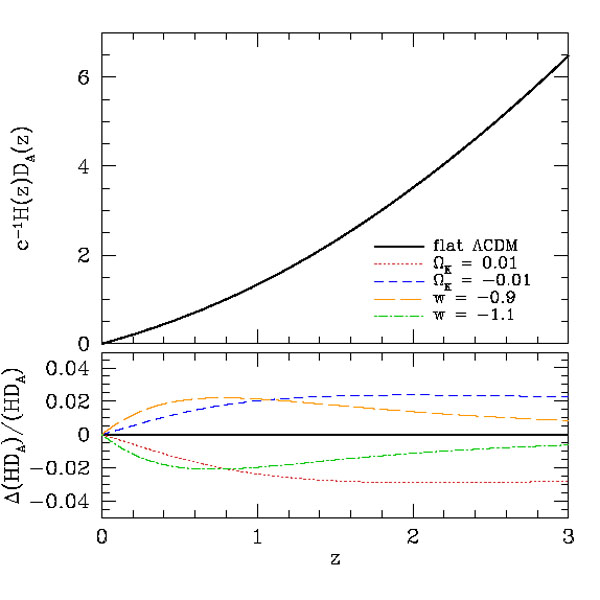Figure 32. Evolution of the parameter combination H(z)DA(z) constrained by the Alcock-Paczynski test, for the same suite of CMB-normalized models shown in Figure 2.

Figure 32 shows the evolution of c^-1 H(z) D_A(z) for the same set of CMB-normalized models shown earlier in Figures 2 - 4. At low redshift, the model dependence resembles that of H(z) / ch (lower left panel of Figure 2), but deviations are reduced in amplitude because of partial cancellation between H(z) and D_A(z) ∝ ∫₀^z dz' H^-1(z'). At high redshift Ω_k = ± 0.01 has a larger impact than 1 + w = ± 0.1. Note that negative space curvature (positive Ω_k) tends to increase D_A, but because the CMB normalization lowers Ω_m (see Table 1) and thus H(z) / H₀, the net effect is to decrease H(z) D_A(z). In Section 8.5.2 we show that our fiducial Stage IV program predicts H(z) D_A(z) with an accuracy of ~ 0.15-0.3%, assuming a w₀ - w_a dark energy model. AP measurements at this level could significantly improve dark energy constraints. For Stage III, the predictions are considerably weaker, ~ 0.5-0.9%.

Like redshift-space distortion measurements, the AP test is automatically enabled by redshift surveys conducted for BAO. In practice the two effects must be modeled together (see, e.g., Matsubara 2004), and the principal systematic uncertainty for AP measurements is the uncertainty in modeling non-linear redshift-space distortions. At present, it is difficult to forecast the likely precision of future AP measurements because there have been no rigorous tests of the accuracy of redshift-space distortion corrections at the level of precision reachable by such surveys. If one assumes that redshift-space distortions can be modeled adequately up to k ~ k_nl then the potential gain from AP measurements is impressively large. For example, Wang et al. (2010) find that using the full galaxy power spectrum in a space-based emission-line redshift survey increases the forecast value of the DETF FoM by a factor of ~ 3 relative to the BAO measurement alone; this gain is not broken down into separate contributions, but we suspect that a large portion comes from AP. ⁷⁰ In the context of HETDEX, Shoji et al. (2009) show that the AP test substantially improves the expected cosmological constraints relative to BAO analysis alone, even after marginalizing over linear RSD and a small-scale velocity dispersion parameter. The appendix to that paper presents analytic formalism for incorporating AP and RSD constraints into Fisher matrix analyses.

Halo occupation methods (see Section 2.3) provide a useful way of approaching peculiar velocity uncertainties in AP measurements. Observations and theory imply that galaxies reside in halos, and on average the velocity of galaxies in a halo should equal the halo's center-of-mass velocity because galaxies and dark matter feel the same large scale acceleration. However, the dispersion of satellite galaxy velocities in a halo could differ from the dispersion of dark matter particle velocities by a factor of order unity, and central galaxies could have a dispersion of velocities relative to the halo center-of-mass (van den Bosch et al. 2005, Tinker et al. 2006). To be convincing, an AP measurement must show that it is robust (relative to its statistical errors) to plausible variations in the halo occupation distribution and to plausible variations in the velocity dispersion of satellite and central galaxies. Alternatively, the AP errors can be marginalized over uncertainties in these multiple galaxy bias parameters, drawing on constraints from the observed redshift-space clustering.

BAO measurements from spectroscopic surveys in some sense already encompass the AP effect, since they use the location of the BAO scale as a function of angular and redshift separations to separately constrain D_A(z) and H(z). The presence of a feature at a particular scale makes the separation of the AP effect from peculiar velocity RSD much more straightforward (see fig. 6 of Reid et al. 2012). However, the addition of a high-precision AP measurement from smaller scales could significantly improve the BAO cosmology constraints. BAO measurements typically constrain D_A(z) better than H(z) because there are two angular dimensions and only one line-of-sight dimension. However, at high redshift H(z) is more sensitive to dark energy than D_A(z), since H(z) responds directly to u_ϕ(z) through the Friedmann equation (3) while D_A(z) is an integral of H₀/H(z') over all z' < z. An AP measurement would allow the BAO measurement of D_A(z) to be "transferred" to H(z), thus yielding a better measure of the dark energy contribution. Blake et al. (2011c) have recently implemented a similar idea by using their AP measurements in the WiggleZ survey to convert SN luminosity distances into H(z) determinations.

The AP test can be implemented with measures other than the power spectrum or correlation function. One option is to use the angular distribution of small scale pairs of quasars or galaxies (Phillipps 1994, Marinoni and Buzzi 2010), though peculiar velocities still affect this measure, in a redshift- and cosmology-dependent way (Jennings et al. 2012b). A promising recent suggestion is to use the average shape of voids in the galaxy distribution; individual voids are ellipsoidal, but in the absence of peculiar velocities the mean shape should be spherical (Ryden 1995, Lavaux and Wandelt 2010). Typical voids are of moderate scale (R ~ 10 h^-1 Mpc) and have a large filling factor f, so the achievable precision in a large redshift survey is high if the sampling density is sufficient to allow accurate void definition. A naive estimate for the error on the mean ellipticity of voids with rms ellipticity є_rms in a survey volume V is σ ~ є_rms (fV / 4/3π R³)^-1/2 ≈ 6 × 10^-4 (є_rms/0.3) (fV / 1 h^-3 Gpc³)^-1/2 (R / 10 h^-1 Mpc)^-3/2, if the galaxy density is high enough to make the shot noise contribution to the ellipticity scatter negligible on scale R. Peculiar velocities have a small, though not negligible, impact on void sizes and shapes (Little et al. 1991, Ryden and Melott 1996, Lavaux and Wandelt 2012), so one can hope that the uncertainty in this impact will be small, but this hope has yet to be tested. Assuming statistical errors only, Lavaux and Wandelt (2012) estimate that a void-based AP constraint from a Euclid-like redshift survey would provide several times better dark energy constraints than the BAO measurement from the same data set, mainly because the scale of voids is so much smaller than the BAO scale. Sutter et al. (2012) have recently applied the AP test to a void catalog constructed from the SDSS DR7 redshift surveys, though with this sample the statistical errors are too large to yield a significant detection of the predicted effect.

7.4. Alternative Distance Indicators

In Sections 3 and 4 we have discussed the two most well established methods for measuring the cosmological distance scale beyond the local Hubble flow: Type Ia supernovae and BAO. These two methods set a high bar for any alternative distance indicators. Type Ia supernovae are highly luminous, making them relatively easy to discover and measure at large distances. Once corrected for light curve duration, local Type Ia's have a dispersion of 0.1-0.15 mag in peak luminosity despite sampling stellar populations with a wide range of age and metallicity, and extreme outliers are apparently rare (Li et al. 2011). Thus far, surveys are roughly succeeding in achieving the √N error reduction from large samples, though progress on systematic uncertainties will be required to continue these gains. The BAO standard ruler is based on well understood physics, and it yields distances in absolute units. "Evolutionary" corrections (from non-linear clustering and galaxy bias) are small and calculable from theory.

Core collapse supernovae exhibit much greater diversity than Type Ia supernovae, which is not surprising given the greater diversity of their progenitors. However, Type IIP supernovae, characterized by a long "plateau" in the light curve after peak, show a correlation between expansion velocity (measured via spectral lines) and the bolometric luminosity of the plateau phase, making them potentially useful as standardized candles with ~ 0.2 mag luminosity scatter (Hamuy and Pinto 2002; see Maguire et al. 2010 for a recent discussion). Unfortunately, as distance indicators Type IIP supernovae appear to be at least slightly inferior to Type Ia supernovae on every score: they are less luminous, the scatter is larger, the fraction of outliers may be larger, and they arise in star-forming environments that are prone to dust extinction. With the existence of cosmic acceleration now well established by multiple methods, we are skeptical that Type IIP supernovae can make a significant contribution to refinement of dark energy constraints.

The door for alternative distance indicators is more open beyond z = 1, the effective limit of most current SN and BAO surveys. Gamma-ray bursts (GRBs) are highly luminous, so they can be detected to much higher redshifts than optical supernovae; the current record holder is at z ≈ 8.2 (Tanvir et al. 2009, Salvaterra et al. 2009). GRBs are extremely diverse and highly beamed, but they exhibit correlations (Amati 2006, Ghirlanda et al. 2006) between equivalent isotropic energy and spectral properties (such as the energy of peak intensity) or variability. These correlations can be used to construct distance-redshift diagrams for those systems with redshift measured via spectroscopy of afterglow emission or of host galaxies (e.g., Schaefer 2007; see Demianski and Piedipalumbo 2011 for a recent review and discussion). While GRBs reach to otherwise inaccessible redshifts, we are again skeptical that they can contribute to our understanding of dark energy because of statistical limitations and susceptibility to systematics. It has taken detailed observations of many hundreds of Type Ia supernovae, local and distant, to understand their systematics and statistics. The number of GRBs with spectroscopic redshifts is ~ 100, and the spectroscopic sample may be a biased subset of the full GRB population because of the requirement of a bright optical afterglow or identified host galaxy.

Quasars are another tool for reaching high redshifts, drawing on empirical correlations between line equivalent widths and luminosity (Baldwin 1977) or between luminosity and the broad line region radius R_BLR (Bentz et al. 2009). For example, Watson et al. (2011) have recently proposed reverberation mapping (which measures R_BLR) of large quasar samples to constrain dark energy models. The high redshift quasar population is systematically different (in black hole mass and host galaxy environment) from lower redshift calibrators. Quasar spectral properties appear remarkably stable over a wide span of redshift (Steffen et al. 2006), and the dependence of R_BLR on luminosity is driven primarily by photoionization physics. However, in the event of a "surprising" result from quasar distance indicators, one would have to be prepared to argue that subtle (e.g., 10% or smaller) changes with redshift were a consequence of cosmology rather than evolution. Of course, quasar distance indicators also face the same challenges of photometric calibration, k-corrections, and dust extinction that affect supernova studies.

Radio galaxies have been employed as a standard (or at least standardizable) ruler for distance-redshift studies, drawing on empirically tested theoretical models that connect the source size to its radio properties (Daly 1994, Daly and Guerra 2002). Analysis of 30 radio galaxies out to z = 1.8 gives results consistent with those from Type Ia supernovae (Daly et al. 2009). The number of radio galaxies to which this technique can be applied is limited, and the model assumptions used to translate observables into distance estimates are fairly complex (see Daly et al. 2009, Section 2.1). We therefore expect that both statistical and systematic limitations will prevent this method from becoming competitive with supernovae and BAO.

In Section 8.5.4 we show forecast distance errors for our fiducial Stage III and Stage IV experimental programs, presenting a target for alternative methods. If one assumes a w₀ - w_a model then the constraints are very tight, with errors below ~ 0.25% at Stage IV and ~ 0.5% at Stage III. However, with a general w(z) model the constraints become much weaker outside the redshift range directly measured by Type Ia SNe or BAO. In particular, our Stage IV forecasts presume large BAO surveys at z > 1, and if these do not come to fruition there is much more room for alternative indicators at high redshift.

7.5. Standard Sirens

Gravitational wave astronomy opens an entirely different route to distance measurement, with an indicator that is grounded in fundamental physics (Schutz 1986). The basic concept is illustrated by considering a nearly Newtonian binary system of two black holes with total mass M and reduced mass μ, in a nearly circular orbit at separation a. The gravitational wave luminosity of such a source is

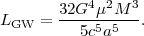(157)

If one can measure the angular velocity of the orbit ⁷¹ = [GM / a³]^1/2, its rate of change due to inspiral as the binary loses energy / ω = 96G³ μ M² / 5c⁵ a⁴, and the orbital velocity v = (GM / a)^1/2 (using relativistic corrections to the emitted waveform), one has enough information to solve for a, M, and μ. One can therefore calculate L_GW from the measured observables and compare to the measured energy flux to infer distance. In practice, one would need to solve for other dimensionless parameters such as the eccentricity and the orientation of the orbit, black hole spins, and source position on the sky. The solution is not trivial (!), but gravitational waveforms from relativistic binaries encode this information in higher harmonics and modulation of the signal due to precession (Arun et al. 2007). Because of the analogy between gravitational wave observations and acoustic wave detection, this approach is often referred to as the "standard siren" method.

There are several practical obstacles to gravitational wave cosmology. First, of course, gravitational waves from an extragalactic source must be detected. The most promising near-term possibility is nearby (z ≪ 1) neutron star binaries, which should be detected by the ground-based Advanced LIGO detector (to start observations in ~ 2014) and upgraded VIRGO detector, and which could be used to measure H₀. The space-based gravitational wave detector LISA (possible launch in the 2020 decade) is designed to allow high S/N measurements of the mergers of massive black holes at the centers of galaxies at z ~ (1), which would enable a full Hubble diagram D_L(z) to be constructed. A second complication is that gravitational wave observations yield a distance but do not give an independent source redshift. One thus needs an identification of the host galaxy, and given the angular positioning accuracy of gravitational wave observations this will generally require identification of an electromagnetic transient that accompanies the gravitational wave burst. Possibilities include GRBs resulting from neutron star mergers (Dalal et al. 2006) and the optical, X-ray, or radio signatures of the response of an accretion disk to a massive black hole merger (Milosavljevic and Phinney 2005, Lippai et al. 2008). However, both the event rates and the characteristics of the electromagnetic signatures are poorly understood at present. One can also make identifications statistically using large scale structure (MacLeod and Hogan 2008). A third complication, important for the high S/N observations expected from LISA, is that weak lensing magnification becomes a dominant source of noise at z ≳ 1, inducing a scatter in distance of several percent per observed source (Markovic 1993, Holz and Linder 2005, Jonsson et al. 2007). By taking advantage of the non-Gaussian shape of the lensing scatter, one can reduce the error on the mean by a factor ~ 2-3 below the naive σ / √N expectation (Hirata et al. 2010, Shang and Haiman 2011), so samples of a few dozen well observed sources could yield sub-percent distance scale errors.

Nissanke et al. (2010) forecast constraints on H₀ from next-generation ground-based gravitational wave detectors, including Monte Carlo simulations of parameter recovery from neutron star-neutron star and neutron star-black hole mergers. They find that H₀ can be constrained to 5% for 15 NS-NS mergers with GRB counterparts and a network of three gravitational wave detectors. While the event rate is highly uncertain, tens of events per year are quite possible and could lead to percent-level constraints on H₀ a decade or so from now. Taylor and Gair (2012) discuss the prospects for a network of "third generation" ground-based interferometers, which could detect ~ 10⁵ double neutron star binaries.

It remains to be seen whether standard sirens can compete with other distance indicators in the LIGO/VIRGO and LISA era. Looking further ahead, Cutler and Holz (2009) show that an interferometer mission designed to search for gravitational waves from the inflation epoch in the 0.03 - 3 Hz range, such as the Big Bang Observer (BBO, Phinney et al. 2004) or the Japanese Decigo mission (Kawamura et al. 2008), would detect hundreds of thousands of compact star binaries out to z ~ 5. The arc-second level resolution would be sufficient to identify the host galaxies for most binaries even at high z, enabling redshift determinations through follow-up observations. With the S/N expected for BBO, the error in luminosity distance for most of these standard sirens would be dominated by weak lensing magnification, and the √N available for beating down this scatter would be enormous. Indeed, Cutler and Holz (2009) argue that the dispersion of distance estimates as a function of separation could itself be used to probe structure growth via the strength of the WL effect. For the BBO case, Cutler and Holz (2009) forecast errors of ~ 0.1%, 0.01, and 0.1 on H₀, w₀, and w_a when combining with a Planck CMB prior, assuming a flat universe. Because the distance indicator is rooted in fundamental physics, there are no obvious systematic limitations to this method provided the calibration of the gravitational wave measurements themselves is adequate.

7.6. The Lyα Forest as a Probe of Structure Growth

The Lyα forest is an efficient tool for mapping structure at z≈ 2-4 because each quasar spectrum provides many independent samples of the density field along its line of sight. (At lower redshifts Lyα absorption moves to UV wavelengths unobservable from the ground, and at higher redshifts the forest becomes too opaque to trace structure effectively.) The relation between Lyα absorption and matter density is non-linear and to some degree stochastic. However, the physics of this relation is straightforward and fairly well understood, in contrast to the more complicated processes that govern galaxy formation. We have previously discussed the Lyα forest as a method of measuring BAO at z > 2, which requires only that the forest provide a linearly biased tracer of the matter distribution on ~ 150 Mpc scales. However, by drawing on a more detailed theoretical description of the forest, one can use Lyα flux statistics to infer the amplitude of matter fluctuations and thus measure structure growth at redshifts inaccessible to weak lensing or clusters.

The Lyα forest is described to surprisingly good accuracy by the Fluctuating Gunn-Peterson Approximation (FGPA, Weinberg et al. 1998; see also Gunn and Peterson 1965, Rauch et al. 1997, Croft et al. 1998), which relates the transmitted flux F = exp(-τ_Lyα) to the dark matter overdensity ρ / , with the latter smoothed on approximately the Jeans scale of the diffuse intergalactic medium (IGM) where gas pressure supports the gas against gravity (Schaye 2001). Most gas in the low density IGM follows a power-law relation between temperature and density, T = T₀(ρ / )^α with α ≲ 0.6, which arises from the competition between photo-ionization heating and adiabatic cooling (Katz et al. 1996, Hui and Gnedin 1997). The Lyα optical depth is proportional to the hydrogen recombination rate, which scales as ρ² T^-0.7 in the relevant temperature range near 10⁴ K. This line of argument leads to the relation

(158)

The constant A depends on a combination of parameters that are individually uncertain (see Croft et al. 1998, Peeples et al. 2010), and the value of α depends on the IGM reionization history, so in practice these parameters must be inferred empirically from the Lyα forest observables. However, even after marginalizing over these parameters there is enough information in the clustering statistics of the flux F to constrain the shape and amplitude of the matter power spectrum (e.g., Croft et al. 2002, Viel et al. 2004, McDonald et al. 2006). Lyα forest surveys conducted for BAO allow high precision measurements of flux correlations on smaller scales, so they have the statistical power to achieve tight constraints on matter clustering.

There are numerous physical complications not captured by equation (158). On small scales, absorption is smoothed along the line of sight by thermal motions of atoms. Peculiar velocities add scatter to the relation between flux and density, though this effect is mitigated if one uses the redshift-space ρ / in equation (158). Gas does not perfectly trace dark matter, so (ρ / )_gas is not identical to (ρ / )_DM. Shock heating and radiative cooling push some gas off of the temperature-density relation. All of these effects can be calibrated using hydrodynamic cosmological simulations, and since the physical conditions are not highly non-linear and the effects are moderate to begin with, uncertainties in the effects are not a major source of concern.

A more serious obstacle to accurate predictions is the possibility that inhomogeneous IGM heating — especially heating associated with helium reionization, which is thought to occur at z ≈ 3 — produces spatially coherent fluctuations in the temperature-density relation that appear as extra power in Lyα forest clustering, or makes the relation more complicated than the power law that is usually assumed (McQuinn et al. 2011, Meiksin and Tittley 2012). Fluctuations in the ionizing background radiation can also produce extra structure in the forest, though this effect should be small on comoving scales below ~ 100 Mpc (McQuinn et al. 2011). On the observational side, the primary complication is the need to estimate the unabsorbed continuum of the quasar, relative to which the absorption is measured. (In our notation, F is the ratio of the observed flux to that of the unabsorbed continuum.) For statistical analysis of a large sample, the continuum does not have to be accurate on a quasar-by-quasar basis, and there are strategies (such as measuring fluctuations relative to a running mean) for mitigating any bias caused by continuum errors (see, e.g., Slosar et al. 2011). Nonetheless, residual uncerainties from continuum determination can be significant compared to the precision of measurements.

A discrepancy between clustering growth inferred from the Lyα forest and cosmological models favored by other data would face a stiff burden of proof, to demonstrate that the Lyα forest results were not biased by the theoretical and observational systematics discussed above. However, complementary clustering statistics and different physical scales have distinct responses to systematics and to changes in the matter clustering amplitude, so it may be possible to build a convincing case. For example, the bispectrum (Mandelbaum et al. 2003, Viel et al. 2004) and flux probability distribution (e.g., Lidz et al. 2006) provide alternative ways to break the degeneracy between mean absorption and power spectrum amplitude and to test whether a given model of IGM physics is really an adequate description of the forest. Lyα forest tests will assume special importance if other measures indicate discrepancies at lower redshifts with the growth predicted by GR combined with simple dark energy models. Growth measurements at z ~ 3 from the Lyα forest could then play a critical role in distinguishing between modified gravity explanations and models with unusual dark energy history. Because it probes high redshifts and moderate overdensities, the Lyα forest can also constrain the primordial power spectrum on small scales that are inaccessible to other methods. The resulting lever arm may be powerful for detecting or constraining the scale-dependent growth expected in some modified gravity models, as discussed further in the next section.

7.7. Other Tests of Modified Gravity

We have concentrated our discussion of modified gravity on tests for consistency between measured matter fluctuation amplitudes and growth rates — from weak lensing, clusters, and redshift-space distortions — with the predictions of dark energy models that assume GR. However, "not General Relativity" is a broad category, and there are many other potentially observable signatures of modified gravity models. For an extensive review of modified gravity theories and observational tests, we refer the reader to Jain and Khoury (2010). We follow their notation and discussion in our brief summary here.

In Newtonian gauge, the spacetime metric with scalar perturbations can be written in the form

(159)

which is general to any metric theory of gravity. If the dominant components of the stress-energy tensor have negligible anisotropic stress, then the Einstein equation of GR predicts that Ψ = Φ, i.e., the same gravitational potential governs the time-time and space-space components of the metric. We have made this assumption implicitly in the WL discussion of Section 5. Anisotropic stress should be negligible in the matter-dominated era, and most proposed forms of dark energy (e.g., scalar fields) also have negligible anisotropic stress. Therefore, one generic form of modified gravity test is to check for the GR-predicted consistency between Ψ and Φ. For example, if the Ricci curvature scalar R in the GR spacetime action S ∝ ∫d⁴ x√-g R is replaced by a function f(R), then Ψ and Φ are generically unequal. In the forecasts of Section 8 we focus on GR-deviations described by the G₉ and Δγ parameters that characterize structure growth (Section 2.2), but an alternative approach parametrizes the ratios of Ψ and Φ to their GR-predicted values (see Koivisto and Mota 2006, Bean and Tangmatitham 2010, Daniel and Linder 2010, and references therein). The G₉ and Δγ formulation is well matched to observables that can be measured by large surveys, but the potentials formulation is arguably closer to the physics of modified gravity.

The main approach to testing the consistency of Ψ and Φ exploits the fact that the gravitational accelerations of non-relativistic particles are determined entirely by Ψ but the paths of photons depend on Ψ + Φ. Thus, an inequality of Ψ and Φ should show up observationally as a mismatch between mass distributions estimated from stellar or gas dynamics and mass distributions estimated from gravitational lensing. (In typical modified gravity scenarios, it is then the lensing measurement that characterizes the true mass distribution.) The approximate agreement between X-ray and weak lensing cluster masses already rules out large disagreements between Ψ and Φ. A systematic statistical approach to this test, employing the techniques discussed in Section 6, could probably sharpen it to the few percent level, limited by the theoretical uncertainty in converting X-ray observations to absolute masses. To reach high precision on cosmological scales, the most promising route is to test for consistency between growth measurements from redshift-space distortions, which respond to the non-relativistic potential Ψ, and growth measurements from weak lensing. Implementing an approach suggested by Zhang et al. (2007), Reyes et al. (2010) present a form of this test that draws on redshift-space distortion measurements of SDSS luminous red galaxies by Tegmark et al. (2006) and galaxy-galaxy lensing measurements of the same population. The precision of the test in Reyes et al. (2010) is only ~ 30%, limited mainly by the redshift-space distortion measurement, but this is already enough to rule out some otherwise viable models. In the long term, this approach could well be pushed to the sub-percent level, with the limiting factors being the modeling uncertainty in redshift-space distortions and systematics in weak lensing calibration. Similar tests on the ~kpc scales of elliptical galaxies have been carried out by Bolton et al. (2006) and Schwab et al. (2010).

Some modified gravity models allow Ψ and Φ to depend on scale and/or time, yielding an "effective" gravitational constant G_Newton → G_Newton(k, t) (where k denotes Fourier wavenumber). Scale-dependent gravitational growth will alter the shape of the matter power spectrum relative to that predicted by GR for the same matter and radiation content. Precise measurements of the galaxy power spectrum shape can constrain or detect such scale-dependent growth. Uncertainties in the scale-dependence of galaxy bias may be the limiting factor in this test, though departures from expectations could also arise from non-standard radiation or matter content or an unusual inflationary power spectrum, and these effects may be difficult to disentangle from scale-dependent growth. The lever arm for determining the power spectrum shape can be extended by using the Lyα forest or, in the long term, redshifted 21cm maps to make small-scale measurements. Time-dependent G_Newton would alter the history of structure growth, leading to non-GR values of G₉ or Δγ, but it could also be revealed by quite different classes of tests. For example, the consistency of big bang nucleosynthesis with the baryon density inferred from the CMB requires G_Newton at t ≈ 1 sec to equal the present day value to within ~ 10% (Yang et al. 1979, Steigman 2010). Variation of G_Newton over the last 12 Gyr would also influence stellar evolution, and it is therefore constrained by the Hertszprung-Russell diagram of star clusters (degl'Innocenti et al. 1996) and by helioseismology (Guenther et al. 1998).

Departures from GR are very tightly constrained by high-precision tests in the solar system, and many modified gravity models require a screening mechanism that forces them towards GR in the solar system and Milky Way environment. ⁷² Screening may be triggered by a deep gravitational potential, in which case the strength of gravity could be significantly different in other cosmological environments. For a generic class of theories, the value of G_Newton would be higher by 4/3 in unscreened environments, allowing order unity effects (see, for example, the discussion of f(R) gravity by Chiba 2003 and DGP gravity by Lue 2006). Chang and Hui (2011) suggest tests with evolved stars, which could be screened in the dense core and unscreened in the diffuse envelope; the stars should be located in isolated dwarf galaxies so that the gravitational potential of the galaxy, group, or supercluster environment does not trigger screening on its own. Hui et al. (2009) and Jain and VanderPlas (2011) propose testing for differential acceleration of screened and unscreened objects in low density environments (e.g., stars vs. gas, or dwarf galaxies vs. giant galaxies), in effect looking for macroscopic and order unity violations of the equivalence principle. Jain (2011) provides a systematic, high-level review of these ideas and their implications for survey experiments, emphasizing the value of including dwarf galaxies at low redshifts within large survey programs.

Evidence for modified gravity could emerge from some very different direction, such as high precision laboratory or solar system tests, tests in binary pulsar systems, or gravity wave experiments. In many of these areas, technological advances allow potentially dramatic improvements of measurement precision — for example, the proposed STEP satellite could sharpen the test of the equivalence principle by five orders-of-magnitude (Overduin et al. 2009). Modified gravity or a dark energy field that couples to non-gravitational forces could also lead to time-variation of fundamental "constants" such as the fine-structure constant α. Unfortunately, there are no "generic" predictions for the level of deviations in these tests, so searches of this sort necessarily remain fishing expeditions. However, the existence of cosmic acceleration suggests that there may be interesting fish to catch.

7.8. The Integrated Sachs-Wolfe Effect

On large angular scales, a major contribution to CMB anisotropies comes from gravitational redshifts and blueshifts of photon energies (Sachs and Wolfe 1967). In a universe with Ω_tot = Ω_m = 1, potential fluctuations δΦ ~ G δ M / R stay constant because (in linear perturbation theory) δ M and R both grow in proportion to a(t). In this case, a photon's gravitational energy shift depends only on the difference between the potential at its location in the last scattering surface and its potential at earth. However, once curvature or dark energy becomes important, δ M grows slower than a(t), potential wells decay, and photon energies gain a contribution from an integral of the potential time derivative ( + in the notation of Section 7.7) known as the Integrated Sachs-Wolfe (ISW) effect. In more detail, one should distinguish the early ISW effect, associated with the transition from radiation to matter domination, from the late ISW effect, associated with the transition to dark energy domination. The ISW effect depends on the history of dark energy, which determines the rate at which potential wells decay. It can also test whether anisotropy is consistent with the GR prediction — in particular whether the Ψ and Φ potentials are equal as expected.

As an observational probe, the ISW effect has two major shortcomings. First, it is significant only on large angular scales, where cosmic variance severely and unavoidably limits measurement precision. (On scales much smaller than the horizon, potential wells do not decay significantly in the time it takes a photon to cross them.) Second, even on these large scales the ISW contribution is small compared to primary CMB anisotropies. The second shortcoming can be partly addressed by measuring the cross-correlation between the CMB and tracers of the foreground matter distribution, which separates the ISW effect from anisotropies present at the last scattering surface. The initial searches, yielding upper limits on Ω_Λ, were carried out by cross-correlating COBE CMB maps with the X-ray background (mostly from AGN, which trace the distribution of their host galaxies) as measured by HEAO (Boughn et al. 1998, Boughn and Crittenden 2004). The WMAP era, combined with the availability of large optical galaxy samples with well-characterized redshift distributions, led to renewed interest in ISW and to the first marginal-significance detections (Fosalba et al. 2003, Scranton et al. 2003, Afshordi et al. 2004, Boughn and Crittenden 2004, Fosalba and Gaztaqaga 2004, Nolta et al. 2004)

Realizing the cosmological potential of the ISW effect requires cross-correlating the CMB with large scale structure tracers over a range of redshifts at the largest achievable scales, and properly treating the covariance arising from the redshift range and sky coverage of each data set. Ho et al. (2008) used 2MASS objects (z < 0.2), photometrically selected SDSS LRGs (0.2 < z < 0.6) and quasars (0.6 < z < 2.0), and NVSS radio galaxies, finding an overall detection significance of 3.7σ. Giannantonio et al. (2008) used a similar sample (but with a different SDSS galaxy and quasar selection, and with the inclusion of the HEAO X-ray background maps) and found a 4.5σ detection of ISW. Both of these measurements are consistent with the "standard" ΛCDM cosmology. ⁷³ Zhao et al. (2010) utilize the Giannantonio et al. (2008) measurement in combination with other data to test for late-time transitions in the potentials Φ and Ψ, finding consistency with GR.

Giannantonio et al. (2008) estimate that a cosmic variance limited experiment could achieve a 7-10σ ISW detection. Because of the low S/N ratio, the ISW effect does not add usefully to the precision of parameter determinations within standard dark energy models, but it could reveal signatures of non-standard models. Early dark energy — dynamically significant at the redshift of matter-radiation equality — can produce observable CMB changes via the early ISW effect (Doran et al. 2007; de Putter et al. 2009 discuss the related problem of constraining early dark energy via CMB lensing). Perhaps the most interesting application of ISW measurements is to constrain, or possibly reveal, inhomogeneities in the dark energy density (see Section 2.2), which produce CMB anisotropies via ISW and are confined to large scales in any case (see de Putter et al. 2010). However, it is not clear whether even exotic models can produce an ISW effect that is distinguishable from the ΛCDM prediction at high significance. Measuring the ISW cross-correlation requires careful attention to angular selection effects in the foreground catalogs, but these effects should be controllable, and independent tracers allow cross-checks of results. Since the prediction of conventional dark energy models is robust compared to expected statistical errors, a clear deviation from that prediction would be a surprise with important implications.

7.9. Cross-Correlation of Weak Lensing and Spectroscopic Surveys

Our forecasts in Section 7.2 incorporate an ambitious Stage IV weak lensing program, and in Section 8.5.3 we consider the impact of adding an independent measurement of f(z) σ₈(z) from redshift-space distortions in a spectroscopic galaxy survey, finding that a 1-2% measurement can significantly improve constraints on the growth-rate parameter Δγ relative to our fiducial program. However, some recent papers (Bernstein and Cai 2011, Gaztaqaga et al. 2012, Cai and Bernstein 2012) suggest that a combined analysis of overlapping weak lensing and galaxy redshift surveys can yield much stronger dark energy and growth constraints than an after-the-fact combination of independent WL and RSD measurements.

The analysis envisioned in these papers involves measurement of all cross-correlations among the WL shear fields (and perhaps magnification fields) in tomographic bins, the angular clustering of galaxies in photo-z bins of the imaging survey, and the redshift-space clustering of galaxies in redshift bins of the spectroscopic survey, as well as auto-correlations of these fields. While the forecast gains emerge from detailed Fisher-matrix calculations, the essential physics (Bernstein and Cai 2011, Gaztaqaga et al. 2012) appears to be absolute calibration of the bias factor of the spectroscopic galaxies via their weak lensing of the photometric galaxies (galaxy-galaxy lensing, Section 5.2.6). This calibration breaks degeneracy in the modeling of RSD, and it effectively translates the spectroscopic measurement of the galaxy power spectrum into a normalized measurement of the matter power spectrum. While the second technique can also be applied to galaxy clustering in the photometric survey, using photo-z's, the clustering measurement in a spectroscopic survey is much more precise because there are more modes in 3-d than in 2-d. The cross-correlation approach is more powerful if the spectroscopic survey includes galaxies with a wide range of bias factors (McDonald and Seljak 2009), e.g., a mix of massive absorption-line galaxies and lower mass emission-line galaxies.

These studies are still in an early phase, and it remains to be seen what gains can be realized in practice. The largest synergistic impact arises when the WL and RSD surveys are comparably powerful in their individual measurements of growth parameters (Cai and Bernstein 2012). Stochasticity in the relation between the galaxy and mass density fields depresses cross-correlations relative to auto-correlations, a potentially important theoretical systematic, though stochasticity is expected to be small at large scales, and corrections can be computed with halo-based models that are constrained by small and intermediate-scale clustering. Conversely, it may be possible to realize these gains even when the weak lensing and spectroscopic surveys do not overlap, by calibrating the bias of a photometric sample that has the same target selection criteria as the spectroscopic sample. Gaztaqaga et al. (2012) also investigate the possibility of implementing these techniques in a narrow-band imaging survey with large numbers of filters, which is effectively a low-resolution spectroscopic survey. They find that most of the gains of a spectroscopic survey are achieved if the rms photo-z uncertainty is Δz / (1 + z) ≲ 0.0035, while larger uncertainties degrade the results.

7.10. Strong Gravitational Lenses

Strong gravitational lenses can be employed to measure expansion history in a variety of ways. One is to simply count the number of lenses as a function of angular separation and (when available) redshift — the predicted counts depend on dark energy because the probability of lensing goes up when path lengths are larger (Kochanek 1996). This approach requires a large sample of lenses with well understood statistical characteristics and selection biases. Observationally it is a stiff challenge, but the more fundamental difficulty is that the predicted counts also depend on the evolution of the mass distribution, in particular that of the early-type galaxies that dominate the lensing statistics. For example, Oguri et al. (2012) derive constraints from a sample of 19 strong lenses found from 50,000+ source quasars in the SDSS, and while the analysis yields a robust detection of dark energy, the cosmological parameter values are significantly degenerate with uncertainties in the evolution of the galaxy velocity function. The latter can be addressed to some degree with measurements of galaxy velocity dispersions, but even then one is left with uncertainty in the exact relation between the observable stellar velocity dispersion and the potential well depth that is important for lensing. With a sufficiently large sample of lenses one can "self-calibrate" by using the full distribution as a function of angular separation and redshift, though one still relies on direct galaxy counts for an overall normalization. While future imaging surveys will yield much larger samples of lens candidates (which can then be confirmed spectroscopically), we suspect that the systematic uncertainties in interpreting lens counts will be too large for this method to be competitive as a dark energy probe — rather, it will probe the dynamical history of galaxy assembly. The number of giant cluster arcs as a function of curvature radius and redshift offers an alternative form of the "lens counting" test that depends on both geometry and structure growth (e.g., Horesh et al. 2011), but one must again understand the detailed mass assembly history of the central regions of massive halos to derive dark energy constraints (Killedar et al. 2012).

A second approach is to use angular positions of multiple sources with different (known) redshifts to obtain distance ratios, a strong-lensing version of the cosmography test discussed in Section 5.2.7. Clusters of galaxies are the best targets for this approach, as they sometimes have large numbers of lensed sources (see Soucail et al. 2004 and Jullo et al. 2010 for representative observational applications). The difficulty is that the sources with different redshifts also probe different locations in the lens potential, so to derive cosmological results one needs strong constraints on substructure in the lens cluster and in the foreground and background mass distributions. Meneghetti et al. (2005) and D'Aloisio and Natarajan (2011) discuss some of the theoretical issues in this approach and their implications for data requirements. Obtaining strong cosmological constraints from cosmographic analysis of cluster lenses will be observationally demanding, and mass modeling uncertainties may be a limiting systematic.

The most promising of the strong-lensing approaches uses time delay measurements, which attach an absolute scale to the angular separations and redshifts measured for a gravitational lens. Predicted time delays scale as H₀^-1, and more generally with the angular diameter distance relation D_A(z). The critical systematic is again the uncertainty in the total mass and mass distribution of the lens, which enters predictions of the angular positions and time delays. Given the observed positions, a time-delay measurement determines a degenerate combination of the distance scale (H₀^-1) and the surface mass density of the lens within the Einstein radius (Kochanek et al. 2003), so a dynamical measurement, usually the stellar velocity dispersion, is required to break the degeneracy and isolate the cosmological information. When the sources are resolved (i.e., galaxies rather than AGN in the optical, or jets mapped with VLBI), or when the multiplicity of images is unusually high, then reproducing the data places more stringent constraints on the mass distributions (e.g., Suyu et al. 2012b). In the best cases, distance scale constraints at the ~ 5% level, after marginalizing over uncertainties in the mass distribution, are achievable for an individual lens (e.g., Suyu et al. 2010, Suyu et al. 2012a). Careful measurements and modeling of a number of well constrained lenses could lead to high aggregate precision, adding significant power to tests of dark energy models (Coe and Moustakas 2009, Linder 2011). The critical question from the point of view of dark energy is whether the mass modeling uncertainties are independent from system to system, so that the net uncertainty drops as 1 / √N, or whether global uncertainties in the approach to mass modeling impose a systematic floor. The answer to this question should become clearer as the current generation of cosmological time-delay analyses proceeds.

7.11. Galaxy Ages

In principle the age of the universe is an observable that can probe cosmic expansion history. The integral that determines age,

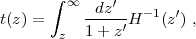(160)

is similar to the integral for comoving distance (eq. 7), except that it extends from z to ∞ instead of 0 to z. The conflict between the ages of globular clusters and the value of t₀ in a decelerating universe was one of the significant early arguments for cosmic acceleration, and a number of authors have employed ages of high-redshift galaxies or clusters of galaxies as a constraint on dark energy models (e.g., Lima and Alcaniz 2000, Jimenez et al. 2003, Capozziello et al. 2004).

Jimenez and Loeb (2002) proposed using differential ages of galaxies at different redshifts to measure, in effect, H(z). Observational studies thus far have concentrated on the massive ellipticals, as these have the fewest complications (dust, ongoing star formation). This differential approach removes some of the uncertainties in the population synthesis models, but it relies on identifying a population of galaxies at one redshift that is just an aged version of a population at a higher redshift, or accounting for the evolutionary corrections that arise from mergers, low-level star formation, and movement of galaxies into or out of the passive population. The state-of-the art observational study is the analysis of ~ 11,000 early-type galaxies from several large surveys by Moresco et al. (2012). They report measurements of H(z) in eight bins out to z ≈ 1, with uncertainties of ~ 5-15% per bin including estimated systematic errors. At low (z < 0.3) redshift, Moresco et al. (2011) analyzed a sample of 14,000 early type galaxies from the SDSS, obtaining H₀ = 72.6 ± 2.9 (stat) ± 2.3 (syst) km s^-1 Mpc^-1, compatible with other estimates of H₀ and competitive in precision. These papers provide extensive discussions of systematic uncertainties and argue that they can be well controlled. Nonetheless, the reliance on population synthesis and galaxy evolution models means that this method will face a stiff burden of proof if it finds a discrepancy with simple dark energy models or other observational analyses, particularly if the differences are at the sub-percent level that is the target of future dark energy experiments.

7.12. Redshift Drift

The redshift of a comoving source changes as the universe expands. Sandage (1962) was the first to propose this "redshift drift" as a cosmological test, but he noted that it appeared far beyond the capabilities of existing experimental techniques. Loeb (1998) repopularized the idea, noting that high-resolution spectrographs on large telescopes could potentially measure the effect in absorption-line spectra of high-redshift quasars. Quercellini et al. (2012) provide an extensive review of the redshift-drift method and other forms of "real-time cosmology" experiments. The expected change in redshift over a time interval Δt, expressed as an apparent velocity shift, is

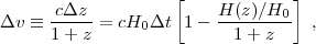(161)

which vanishes for a coasting universe with H(z) / H₀ = (1 + z)^-1. For our fiducial cosmological model, the predicted change over a Δt = 10 year observational span is +1.32 cm s^-1, -1.21 cm s^-1, and -3.66 cm s^-1 for sources at z = 2, 3, and 4, respectively. Corasaniti et al. (2007) estimate that observations of 240 quasars over a span of 30 years using the CODEX spectrograph proposed for the European Extremely Large Telescope could measure H(z) over z = 2-5 with an aggregate precision of ≈ 2% (see Liske and Codex Team 2006 and Balbi and Quercellini 2007 for similar discussions and Liske et al. 2008 for detailed calculations of CODEX performance). The BAO component of the fiducial Stage IV program that we present in Section 8.1 (which assumes 25% sky coverage and errors that are 1.8 times those of linear theory sample variance) yields errors of 0.6-0.7% in H(z) per bin of 0.07 in ln(1 + z) at z = 2-3 (see Table 6). The fiducial BAO program would thus be much more powerful than the redshift-drift approach, but it is not yet clear that high-redshift BAO surveys of this volume will prove practical.

7.13. Alternative Methods: Summary

Of the methods described in this section, redshift-space distortion is the one that seems almost guaranteed to have a broad-ranging impact in future studies of cosmic acceleration. Because of its direct sensitivity to f(z) and its use of non-relativistic tracers, RSD is a valuable complement to weak lensing and clusters as a probe of structure growth. The redshift surveys ongoing or planned for BAO measurements will automatically enable RSD measurements with high statistical precision over a significant range in redshift. The primary systematics for RSD are associated with theoretical modeling uncertainties, and these are likely to diminish with time as more sophisticated techniques are developed, numerical simulations become more powerful, and galaxy clustering measurements provide more detailed tests of the models. The AP method may also amplify the return from BAO redshift surveys, perhaps by a large factor, depending on the success of modeling non-linear velocity distortions.

The z = 0 Hubble constant is only a single number, but it is an important one, as it determines the current critical density and the current expansion rate, with the maximal leverage against the CMB at z ≈ 1100. Ongoing technical developments seem to offer a realistic path to achieving H₀ measurements with 1-2% uncertainty, tight enough to make significant contributions to dark energy constraints even in the era of Stage IV experiments. JWST and Gaia represent dramatic improvements in technological capabilities for H₀ studies, perhaps allowing progress to the sub-percent level.

The impact of the other methods discussed here is more difficult to predict. In some cases, interesting results at the few-percent level are already in hand but it is still too early to say whether the limiting systematics can be reduced to the percent or sub-percent level required for long-term progress. In other cases, such as precision gravity tests, there are clear paths to radically improved measurements, but these will provide useful clues or tests only for a limited class of cosmic acceleration models.

The one method that looks like it could ultimately outperform even Stage IV experiments is that of standard sirens applied to compact star binaries (Section 7.5), because of the opportunity to measure hundreds of thousands of distances by a technique that has no obvious limiting systematics. This approach requires extraordinary technological advances, which are unlikely to be achieved in the next decade, and perhaps not in the next two decades. However, the most precise mapping of the expansion history of the universe might ultimately come from spacetime ripples rather than electromagnetic waves.

⁶⁹ We caution that the space densities assumed by White et al. (2009) are much higher than those that Euclid or WFIRST is likely to achieve, so these RSD precision forecasts may prove overoptimistic. Recent forecasts in the specific context of Euclid and WFIRST appear in Majerotto et al. (2012) and Green et al. (2012), respectively. Back.

⁷⁰ Since RSD and AP both depend on modeling the broadband P(k, μ), it is difficult even in principle to separate the two types of constraints in an observational analysis. Back.

⁷¹ The observed frequency of the gravitational wave is 2ω because the source is a quadrupole, producing two crests and two troughs per orbit. Back.

⁷² To give one example, the Shapiro delay of radio waves passing near the Sun, measured to agree with GR to five decimal places (Bertotti et al. 2003), is reduced in theories of gravity that contain scalar fields, but the effect could be suppressed by scalar self-interaction in dense environments. Back.

⁷³ The Ho et al. (2008) measurement is almost 2σ above ΛCDM, but we attribute no special significance to this! Back.