


Having discussed many observational methods individually, we now turn to what we might hope to learn from them in concert. To the extent that this report has an underlying editorial theme, it is the value of a balanced observational program that pursues multiple techniques at comparable levels of precision. In our view, there is much more to be gained by doing a good job on three or four methods than by doing a maximal job on one at the expense of the others. This is not a "try everything" philosophy — moving forward from where we are today, an observational method is interesting only if it has reasonable prospects of achieving percent- or sub-percent-level errors, both statistical and systematic, on observables such as H(z), D(z), and G(z). The successes of cosmic acceleration studies to date have raised the field's entry bar impressively high.
A balanced strategy is important both for cross-checking of systematics and for taking advantage of complementary information. Regarding systematics, the next generation of cosmic acceleration experiments seek much higher precision than those carried out to date, so the risk of being limited or biased by systematic errors is much higher. Most methods allow internal checks for systematics — e.g., comparing distinct populations of SNe, measuring angular dependence and tracer dependence of BAO signals, testing for B-modes and redshift-scaling of WL — but conclusions about cosmic acceleration will be far more convincing if they are reached independently by methods with different systematic uncertainties. Two methods only provide a useful cross-check of systematics if they have comparable statistical precision; otherwise a result found only in the more sensitive method cannot be checked by the less sensitive method.
Regarding information content, we have already emphasized the complementarity of SN and BAO as distance determination methods. SN have unbeatable statistical power at z ≲ 0.6, while BAO surveys that map a large fraction of the sky with adequate sampling can achieve higher precision at z ≳ 0.8. Overlapping SN and BAO measurements provide independent physical information because the former measure relative distances and the latter absolute distances (h-1 Mpc vs. Mpc), and the value of h is itself a powerful dark energy diagnostic in the context of CMB constraints (see Section 7.1 and Section 8.5.1). WL, clusters, and redshift-space distortions provide independent constraints on expansion history, at levels that can be competitive with SN and BAO, and they provide sensitivity to structure growth. Without structure probes, we would have little hope of clues that might locate the origin of acceleration in the gravitational sector rather than the stress-energy sector, and we would, more generally, reduce the odds of "surprises" that might push us beyond our current theories of cosmic acceleration.
The primary purpose of this section is to present quantitative forecasts for a program of Stage IV dark energy experiments and to investigate how the forecast constraints depend on the performance of the individual components of such a program. Our forecasts are analogous to those of the DETF (Albrecht et al. 2006), updated with a more focused idea of what a Stage IV program might look like, and updated in light of subsequent work on parameterized models and figures of merit for dark energy experiments, most directly that of the JDEM Figure-of-Merit Science Working Group (FoMSWG; Albrecht et al. 2009). In Section 8.1 we summarize our assumptions about the fiducial program. In Section 8.2 we describe the methodology of our forecasts, in particular the construction of Fisher matrices for the fiducial program. In Section 8.3 we present results for the fiducial program and for variants in which one or more components of this program are made significantly better or worse. We also compare these results to forecasts of a "Stage III" program represented by experiments now underway or nearing their first observations.
We have elected to focus on SN, BAO, and WL as the components of these forecasts, for two reasons. First, it is more straightforward (though still not easy) to define the expected statistical and systematic errors for these methods than for others. Second, the most promising alternative methods — clusters, redshift-space distortions, and the Alcock-Paczynksi effect — will be enabled by the same data sets obtained for WL and BAO studies. It is therefore reasonable to view these as auxiliary methods that may improve the return from these data sets (perhaps by substantial factors) rather than as drivers for the observational programs themselves. In Sections 8.4 and 8.5 we present forecasts for how well the fiducial CMB+SN+BAO+WL programs predict the observables of these and other alternative methods, providing a target for how well they must perform to add new information beyond that in our primary probes. In some cases we find that plausible levels of performance could substantially improve tests of cosmic acceleration models. In Section 8.6 we focus on the precision with which our fiducial program measures fundamental observables, and we discuss aggregate precision as a useful, nearly model-independent way of characterizing the power of an experiment and the level of systematics control required to realize it. Section 8.7 provides a high-level summary, discussing the potential yield from programs that combine CMB, SN, BAO, and WL measurements with additional constraints from clusters, redshift-space distortions, and direct H0 determinations.
As discussed in Section 1.3, Astro2010 and the European Astronet report have placed high priority on ground- and space-based dark energy experiments. The Stage III experiments currently underway will already allow much stronger tests of cosmic acceleration models, and Stage IV facilities built over the next decade should advance the field much further still. Our Stage IV program corresponds roughly to the goals recommended by the Cosmology and Fundamental Physics panel report of Astro2010.
For SN studies, we anticipate that Stage IV efforts will be limited not by statistical errors but by systematics associated with photometric calibration, dust extinction, and evolution of the SN population. For our fiducial program, we assume that SN surveys will achieve net errors (statistical + systematic) of 0.01 mag for the mean distance modulus in each of three redshift bins of width Δz = 0.2 extending from z = 0.2 to a maximum redshift zmax = 0.8 (see discussion in Section 3.4). We also assume the existence of a local SN sample at z = 0.05 with the same 0.01 mag net error. High quality observations could yield a smaller systematic error in the local sample, but we suspect that the most challenging systematic for this local calibration will be transferring it to the more distant bins. We treat the bin-to-bin errors as uncorrelated, though this is clearly an approximation to systematic errors that are correlated at nearby redshifts and gradually decorrelate as one considers differing redshift ranges and observed-frame wavelengths. Even with 0.15 mag errors per SN, achieving this level of statistical error requires only 225 SNe per bin, and we expect that the error per SN can be reduced by working at red/IR wavelengths and by selecting sub-populations based on host galaxy type, spectral properties, and light curve shape. For purely ground-based efforts, we consider our 0.01 mag floor for systematic errors to be somewhat optimistic, given the challenges of dust extinction corrections and photometric calibration. However, a space-based program at rest-frame near-IR wavelengths, enabled by WFIRST, could plausibly achieve better than 0.01 mag systematics. We suspect that it will be hard to push calibration and evolution systematics below 0.005 mag even with WFIRST, and pushing statistical errors below this level begins to place severe demands on spectroscopic capabilities, unless purely photometric information can be used to identify populations with scatter below 0.1 mag per SN. We also consider the impact of increasing zmax beyond 0.8, though we argue that this is beneficial mainly when one is hitting a systematics floor at lower z and high-z observations have uncorrelated systematics.
For BAO, the primary metric of statistical constraining power is the total comoving volume mapped spectroscopically with a sampling density high enough to keep shot-noise sub-dominant. There are several projects in the planning stages that could map significant fractions of the comoving volume available out to z ≈ 3. These include the near-IR spectroscopic components of Euclid and WFIRST, ground-based optical facilities such as BigBOSS, DEspec, and SuMIRe PFS, and radio intensity-mapping experiments (see Section 4.7). For our fiducial program, we assume that these projects will collectively map 25% of the comoving volume out to z = 3, with errors a factor of 1.8 larger than the linear theory sample variance errors. 74 We specifically assume full redshift coverage from z = 0-3 with fsky = 25% sky fraction, but other combinations of redshift coverage and fsky that have the same total comoving volume yield similar results. The factor 1.8 accounts for imperfect sampling (hence non-negligible shot-noise) and for non-linear degradation of the BAO signal. It approximates the effects of sampling with nP=2 and using reconstruction (Section 4.3.3) to remove 50% but not 100% of the non-linear Lagrangian displacement of tracers. We implicitly assume that theoretical systematics associated with location of the BAO peak will remain below this level, an assumption we consider reasonable but not incontrovertible based on the discussion in Section 4.5.
For WL, the primary metric of statistical constraining power is the total number of galaxies that have well measured shapes and good enough photometric redshifts to allow accurate model predictions and removal of intrinsic alignment systematics. For our fiducial case, we assume a survey of 104 deg2 achieving an effective surface density of 23 galaxies per arcmin2 with zmed = 0.84, corresponding to Iab < 25 and reff > 0.25". The effective galaxy number is 8.3 × 10⁸. Euclid plans a 14,000 deg2 imaging survey and can likely achieve this surface density or slightly higher. LSST will survey a still larger area, and it might or might not achieve this effective surface density, depending on how low a value of reff / rpsf it can work to before shape measurements are systematics dominated. The WFIRST design reference mission (Green et al. 2012; DRM1) would achieve neff ≈ 40 arcmin-2 but would only image 3400 deg2 in its 2.4-year high-latitude survey, thus measuring about 4.8 × 10⁸ galaxy shapes. An extended WFIRST mission, or an implementation of WFIRST using one of the NRO 2.4-m telescopes (Dressler et al. 2012), could potentially reach 104 deg2. Even individually, therefore, any one of these projects may well exceed the number of shape measurements assumed in our fiducial program, and collectively they will almost certainly do so. We compute constraints from cosmic shear in 14 bins of photometric redshift and from the shear-ratio test described in Section 5.2.7, but we do not incorporate higher order lensing statistics or galaxy-shear cross-correlations. We include information up to multipole lmax = 3000, beyond which statistical power becomes limited at this surface density and systematic uncertainties associated with non-linear evolution and baryonic effects become significant.
Forecasting the systematic uncertainties in Stage IV WL experiments is very much a shot in the dark. Systematic errors are already comparable to statistical errors in surveys of 100 deg2, so lowering them to the level of statistical errors in a 104 deg2 survey that has higher galaxy surface density requires more than an order of magnitude improvement. We therefore consider a "fiducial" and an "optimistic" case for WL systematics. For the fiducial case, we incorporate (and marginalize over) aggregate uncertainties of 2 × 10⁻³ in shear calibration and 2 × 10⁻³ in the mean photo-z, with errors in each redshift bin larger by √14 but uncorrelated across bins. We also incorporate intrinsic alignment uncertainty as described by Albrecht et al. (2009, Section 2h of Appendix A), which includes marginalization over both GI and II components (see Section 5.6.1). For our "optimistic" case we adopt no specific form of the systematic errors but simply assume that they will double the statistical errors throughout. At an order of magnitude level, we can see that the optimistic case corresponds to a global fractional error σ ~ 2 Nmode-1/2 ~ 2 fsky-1/2 lmax-1 = 1.3 × 10⁻³, significantly lower than the fiducial case assumption of 2 × 10⁻³ errors for shear and photo-z calibration (which, roughly speaking, combine in quadrature to make a 2.8 × 10⁻³ multiplicative uncertainty). However, at scales and redshifts where the statistical errors are large, multiplying them by two can be a larger change than adding the shear-calibration and photo-z systematics. As a result, there will be some measures (e.g., the error on Ωk) for which our "optimistic" program performs slightly worse than our fiducial program. Of course, WL experiments that achieved the statistical limits of several × 109 source galaxies — possible in principle — would be several times more powerful than even our optimistic scenario.
The fiducial program outlined above provides a baseline for evaluating improvement in the determination of the cosmological parameters relative to current constraints. We use a Fisher matrix analysis to quantify this improvement and to study the complementarity of the main probes of cosmic acceleration. Since our knowledge of the exact design of future surveys and the systematic errors they will face is inherently imperfect, we also consider the effect of varying the precision of each technique in our forecasts, including both pessimistic and optimistic cases for SN, BAO, and WL data.
Quantifying the impact of each probe on our understanding of cosmic acceleration requires metrics for evaluating progress. The precision with which the dark energy equation of state (and its possible time dependence) can be measured is a common choice; while not the only quantity of interest, it is clearly a central piece of the puzzle. One of the main quantities we use below is the DETF figure of merit defined in equation (26), FoM = [σ(wp) σ(wa)]-1. The FoM indicates how well an experiment determines the dark energy equation of state parameter and its derivative dw / da at the pivot redshift zp, and it thereby indicates the ability to detect deviations from the standard ΛCDM model with wp = -1 and wa = 0. When one considers experiments of increasing power, σ(wp) and σ(wa) tend to shrink in concert, so the DETF FoM scales roughly as an inverse variance and therefore increases linearly with data volume when statistical errors dominate. If the error of every individual measurement (e.g., each DL or H(z) measurement) goes down by √2, then the FoM doubles.
While the DETF FoM is relatively simple to evaluate for a particular experiment, it omits much of the information that will be available from future experiments, including some potentially important clues to the nature of cosmic acceleration. For example, the true dark energy dynamics may be considerably more complicated than what the two-parameter linear model can accommodate, so that constraints on w0 and wa may yield incomplete or misleading results. Additionally, the equation of state alone is insufficient to describe the full range of possible alternatives to the standard cosmological model. For example, modified gravity theories can mimic the effect of any particular equation of state evolution on the Hubble expansion rate and the distance-redshift relation while altering the rate of growth of large-scale structure (e.g., Lue et al. 2004, Song et al. 2007). Including such possibilities requires extra parameters that describe changes in the growth history that are independent of equation of state variations, as discussed in Section 2.2. Other standard parameters of the cosmological model, such as the spatial curvature and the Hubble constant, are important due to degeneracies with the effects of cosmic acceleration that can limit the precision of constraints on the dark energy equation of state.
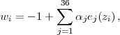
To include more general variations of the equation of state as well as altered growth of structure from modifications to GR on large scales, we adopt the JDEM FoMSWG parameterization (Albrecht et al. 2009). The equation of state in this parameterization is allowed to vary independently in each of 36 bins of width Δa = 0.025 extending from the present to a = 0.1 (z = 9). Specifically, the equation of state has a constant value of wi at (1 - 0.025i) < a < [1 - 0.025(i-1)], for i = 1,…,36. At earlier times, the equation of state is assumed to be w = -1, although the impact of this assumption is typically quite small since dark energy accounts for a negligible fraction of the total density at z > 9 in most models. Modifications to the linear growth function of GR GGR(z) are included through the parameters G9 and Δγ as defined in equations (44) and (45). These parameters describe the change relative to GR in the normalization of the growth of structure at z = 9 and in the growth rate at z < 9, respectively. Adding these to the binned wi values and the standard ΛCDM parameters, the full set is
 |
(162) |
where the primordial amplitude As is defined at
k = 0.05 Mpc-1.
Δ is an overall
offset in the absolute magnitude scale of Type Ia supernovae.
The Hubble constant is determined by these parameters through
h2 =
Ωm h2 +
Ωk h2 +
Ωϕ h2.
We compute our forecasts at the fiducial parameter values chosen by
the FoMSWG to match CMB constraints from the 5-year release of WMAP data
(Komatsu et
al. 2009);
these are listed in Table 5.
These parameters are similar but not identical to those of
the model used in Section 2
(Table 1), which is based on WMAP7.
Note that spatially
flat ΛCDM and GR are assumed for the fiducial model.
is an overall
offset in the absolute magnitude scale of Type Ia supernovae.
The Hubble constant is determined by these parameters through
h2 =
Ωm h2 +
Ωk h2 +
Ωϕ h2.
We compute our forecasts at the fiducial parameter values chosen by
the FoMSWG to match CMB constraints from the 5-year release of WMAP data
(Komatsu et
al. 2009);
these are listed in Table 5.
These parameters are similar but not identical to those of
the model used in Section 2
(Table 1), which is based on WMAP7.
Note that spatially
flat ΛCDM and GR are assumed for the fiducial model.
| w1 | ... | w36 | lnG9 | Δγ | Ωm h2 | Ωb h2 | Ωk h2 | Ωϕ h2 | lnAs | ns | Δ |
| -1 | ... | -1 | 0 | 0 | 0.1326 | 0.0227 | 0 | 0.3844 | -19.9628 | 0.963 | 0 |
We use a Fisher matrix analysis to estimate the constraints on these parameters from the fiducial program defined in Section 8.1 and its variations. The Fisher matrix for each experiment consists of a model of the covariance matrix for the observable quantities and derivatives of these quantities with respect to the parameters. We compute the latter numerically with finite differences and confirm the results using analytic expressions when possible.
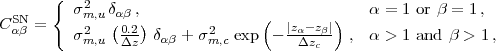
We model SN data as measurements of the average SN magnitude in each of several redshift bins and in a low-redshift calibration sample. While our fiducial case assumes that the net magnitude error is uncorrelated from one bin to the next, we also consider the impact of including a correlated component of the error by defining the SN covariance matrix as
 |
(163) |
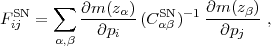
where Δz is the bin width, σm,u is the uncorrelated error in a bin of width Δz = 0.2 (or in the local sample at redshift z1), σm,c is the correlated error with correlation length Δzc, and the net error in each bin zα (α > 1) is σm = (σm,u2 + σm,c2)1/2. In general these errors are redshift dependent, but here we assume that they are constant for simplicity. We do not consider possible correlations between the local SN sample and the high-redshift bins. For the fiducial forecasts we take σm,c = 0, so the covariance matrix is diagonal. The SN Fisher matrix is then computed as a sum over redshift bins
 |
(164) |
where m(zα) =
5log[H0
< DL(zα)>]
+
is the average magnitude in the bin and the
derivatives are taken with respect to the parameters of equation (162).
| zmin | zmax | V [(Gpc / h)3] | σln(D / rs) [%] | σln(Hrs) [%] |
| 0.000 | 0.072 | 0.010 | 13.386 | 21.881 |
| 0.072 | 0.149 | 0.075 | 4.895 | 8.002 |
| 0.149 | 0.231 | 0.217 | 2.873 | 4.697 |
| 0.231 | 0.320 | 0.449 | 1.997 | 3.265 |
| 0.320 | 0.414 | 0.781 | 1.515 | 2.476 |
| 0.414 | 0.516 | 1.218 | 1.213 | 1.983 |
| 0.516 | 0.625 | 1.761 | 1.009 | 1.649 |
| 0.625 | 0.741 | 2.407 | 0.863 | 1.410 |
| 0.741 | 0.866 | 3.148 | 0.754 | 1.233 |
| 0.866 | 1.000 | 3.970 | 0.672 | 1.098 |
| 1.000 | 1.144 | 4.860 | 0.607 | 0.992 |
| 1.144 | 1.297 | 5.799 | 0.556 | 0.909 |
| 1.297 | 1.462 | 6.770 | 0.514 | 0.841 |
| 1.462 | 1.639 | 7.758 | 0.481 | 0.785 |
| 1.639 | 1.828 | 8.745 | 0.453 | 0.740 |
| 1.828 | 2.031 | 9.718 | 0.429 | 0.702 |
| 2.031 | 2.249 | 10.664 | 0.410 | 0.670 |
| 2.249 | 2.482 | 11.576 | 0.393 | 0.643 |
| 2.482 | 2.732 | 12.443 | 0.379 | 0.620 |
| 2.732 | 3.000 | 13.261 | 0.368 | 0.601 |
| Column 3 gives the volume of the redshift slice for fsky = 0.25. In all redshift slices, errors on D / rs and Hrs are correlated with correlation coefficient r = 0.409. | ||||
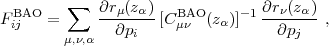
For BAO we divide the observed volume into bins of equal width in ln(1 + z), assumed to be uncorrelated, and compute the Fisher matrix
 |
(165) |
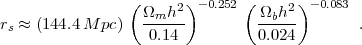
where the measurement vector r(zα) ≡ {D(zα) / rs, H(zα) rs}, the sum is over μ,ν = 1,2 and α = 1,...Nbin, and rs is the sound horizon at recombination (see Section 2.3), for which we use the fitting formula from Hu (2005),
 |
(166) |
We estimate the covariance matrix in each redshift bin using the BAO forecast code by Seo and Eisenstein (2007), which provides estimates of the fractional error on distance and the Hubble expansion rate at each redshift (relative to rs), σln(D / rs) = [C11BAO]1/2 / (D / rs) and σln(Hrs) = [C22BAO]1/2 / (Hrs), respectively, as well as the cross correlation r = C12BAO / [C11BAO C22BAO]1/2. For our default forecasts, we start with the linear theory cosmic variance predictions, corresponding to the limit of perfect sampling of the density field within the observed volume and no degradation of the signal due to nonlinear effects. To approximate the effects of finite sampling and nonlinearity, we increase these errors by a factor of 1.8 for our fiducial forecasts, which leads to parameter constraints comparable to what would be expected with sampling nP = 2 and reconstruction that halves the effects of nonlinear evolution. In Table 6 we list the volume for fsky = 0.25 and fiducial BAO covariance matrix elements for 20 redshift slices from 0≤ z ≤ 3. The results we obtain are only weakly dependent on the number of redshift bins chosen to divide up the total volume.
The WL Fisher matrix is based on the methodology described by Albrecht et al. (2009), where the explicit formulas are given. It includes both power spectrum tomography and cross-correlation cosmography (redshift scaling of the galaxy-galaxy lensing signal), but makes no assumption about the galaxy bias. The galaxies are sliced into Nz = 14 redshift bins and we consider power spectra in Nℓ = 18 bins logarithmically spaced over 10 < ℓ < 104. We consider all power spectra and cross-spectra of the galaxies gi and the E-mode shear γiE. This leads to 2Nz scalar fields on the sky, and hence N2pt = 2Nz(2Nz + 1) / 2 × Nℓ bins in the power spectrum matrix. 75 The length N2pt vector C of power spectra incorporates all 2-point information.
Our task is now to construct a model both for C and for its covariance matrix Σ, and then to construct the Fisher matrix for parameters p:
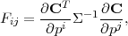 |
(167) |
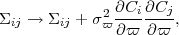
where T denotes a matrix transpose. Systematic errors may be incorporated as either nuisance parameters p (marginalized over some prior) or as additional contributions to Σ:
 |
(168) |
where ϖ is the amplitude of some systematic and σϖ is the amount over which it is marginalized.
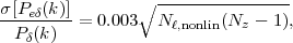
We incorporate in Σ the following contributions:
 |
(169) |
where the square root is introduced to prevent many bins from being used to "average down" this systematic (Albrecht et al. 2009)
The photometric redshift errors (one bias parameter for each bin) and shear calibration errors (also one bias parameter for each bin) are treated as nuisance parameters in the parameter vector p and are marginalized out before combining with other cosmological probes.
The forecasts for the main SN, BAO, and WL probes are supplemented by the expected constraints from upcoming CMB measurements provided by the Planck satellite. We adopt the Fisher matrix FCMB constructed by the FoMSWG, which includes cosmological constraints from the 70, 100, and 143 GHz channels of Planck with fsky = 0.7, assuming that data collected at other frequencies will be used for foreground removal. The noise level and beam size for each channel comes from the Planck Blue Book (Planck Collaboration 2006). Information from secondary anisotropies of the CMB is not included in this Fisher matrix; in particular, constraints from the ISW effect (Section 7.8) are removed by requiring the angular diameter distance to the CMB to be matched exactly, as described in Albrecht et al. (2009). Additionally, the large-scale (ℓ < 30) polarization angular power spectrum and temperature-polarization cross power spectrum, which mainly contribute to constraints on the optical depth to reionization τ, are excluded from the forecast and replaced by a Gaussian prior with width στ = 0.01. This prior accounts for uncertainty in τ due to limited knowledge of the redshift dependence of reionization, which is not included in the simplest models of the CMB anisotropies. Although τ does not appear in the parameter set for the Fisher matrices, marginalization over τ in the CMB constraints contributes to the uncertainty on the primordial power spectrum amplitude As, which in turn affects predictions for the growth of large-scale structure.
Combined constraints on cosmological parameters are obtained simply by adding the Fisher matrices of the individual probes, i.e. F = FSN + FBAO + FWL + FCMB. Then the forecast for the parameter covariance is C = F-1, and in particular the uncertainty on a given parameter pi after marginalizing over the error on all other parameters is ([F-1]ii)1/2.
Computing the Fisher matrix in the FoMSWG parameter space with a large number of independent bins for w(z) gives us the flexibility to project these forecasts onto a number of simpler parameterizations, including the w0 - wa model for the purposes of computing the FoM. To change from the original parameter set p to some new set q, we compute
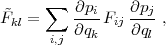 |
(170) |
which gives the Fisher matrix
 for the new
parameterization. In particular, projection from bins
wi to w0 and wa
involves the derivatives
∂ wi
/ ∂ w0 = 1 and
∂ wi
/ ∂ wa = z / (1 + z). We also
compute the pivot redshift zp and the uncertainty in
the equation of state at that redshift,
wp. Given the 2 × 2 covariance matrix
Cij
for w0 and wa (marginalized over the
other parameters), the pivot values are computed as
(Albrecht et
al. 2009)
for the new
parameterization. In particular, projection from bins
wi to w0 and wa
involves the derivatives
∂ wi
/ ∂ w0 = 1 and
∂ wi
/ ∂ wa = z / (1 + z). We also
compute the pivot redshift zp and the uncertainty in
the equation of state at that redshift,
wp. Given the 2 × 2 covariance matrix
Cij
for w0 and wa (marginalized over the
other parameters), the pivot values are computed as
(Albrecht et
al. 2009)
 |
(171) |
where the first index corresponds to w0 and the second to wa.
One drawback to the w0 - wa parameterization is that constraints on w(z) at high redshift are coupled to those at low redshift by the form of the model; for example, if observations determine the value of the equation of state perfectly at z = 0 and at z = 0.1, then it is completely determined at high redshift even in the absence of high redshift data. To specifically address questions related to the ability of dark energy probes to constrain dark energy at low redshift vs. high redshift, we define an alternative but equally simple parameterization in which w(z) takes constant, independent values in each of two bins at z ≤ 1 and z > 1. The projection onto this parameterization using equation (170) requires the derivatives ∂ wi / ∂ w(z ≤ 1) = Θ(1 - zi) and ∂ wi / ∂ w(z > 1) = 1 - Θ(1 - zi), where Θ(x) is the Heaviside step function equal to 0 for x < 0 and 1 for x ≥ 0.
Principal components (PCs) of the dark energy equation of state provide another way to determine which features of the equation of state evolution are best constrained by a given combination of experiments (Huterer and Starkman 2003, Hu 2002a, Huterer and Cooray 2005, Wang and Tegmark 2005, Dick et al. 2006, Simpson and Bridle 2006, de Putter and Linder 2008, Tang et al. 2011, Crittenden et al. 2009, Mortonson et al. 2009b, Kitching and Amara 2009, Maturi and Mignone 2009). We compute the PCs for each forecast case by taking the total Fisher matrix for the original parameter set (eq. 162) and marginalizing over all parameters other than the 36 binned values of wi. If we call the Fisher matrix for the wi parameters Fw, then the PCs are found by diagonalizing Fw:
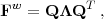 |
(172) |
where Q is an orthogonal matrix whose columns are eigenvectors of Fw and Λ is a diagonal matrix containing the corresponding eigenvalues of Fw. Up to an arbitary normalization factor, the eigenvectors are equal to the PC functions ei = (ei(z1), ei(z2), ...) which describe how the binned values of w(z) are weighted with redshift. Here we adopt the normalization of Albrecht et al. (2009),
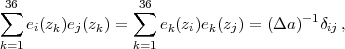 |
(173) |
where Δa = 0.025 is the bin width; for i = j this condition approximately corresponds to ∫0.11 da [ei(a)]2 = 1. With this convention, the columns of Q are (Δa)1/2 ei. The PCs rotate the original set of parameters to a set of PC amplitudes QT (1 + w) with elements
 |
(174) |
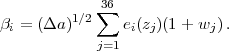
Combining equations (173) and (174), we can construct w(z) in each redshift bin from a given set of PC amplitudes as
 |
(175) |
where αi ≡ (Δa)1/2 βi. The accuracy with which the αi can be determined from the data is given by the eigenvalues of Fw, σi ≡ σαi = (Δa / Λii)1/2, and the PCs are numbered in order of increasing variance (i.e. σi+1 > σi).
For constraints that are marginalized over the wi parameters, we impose a weak prior on wi as suggested by Albrecht et al. (2009) to reduce the dependence of forecasts for Δγ on the poorly-constrained high redshift wi values, since arbitrarily large fluctuations in w(z) can alter the high redshift growth rate. We include a weak Gaussian prior with width σwi = Δw / √Δa by adding to the total Fisher matrix
 |
(176) |
assuming that the parameters are ordered as in equation (162) with p1 = w1, p2 = w2, etc. For most forecasts, we use a default prior width of Δw = 10 (σwi ≈ 63), which approximately corresponds to requiring that the average value of |1 + w| in all bins does not exceed 10. In the next section we also consider how constraints on certain parameters change with a narrower prior of Δw = 1. For priors wider than the default choice, the Fisher matrix computations are subject to numerical effects arising from the use of a finite number of wi bins to approximate continuous variations in w(z), so we do not present results with weaker priors than Δw = 10. Note that the construction of PCs of w(z) as described above does not include such a prior on wi.
| Any × 4 | Quadruple fiducial errors (divide Fisher matrix by 16). |
| Any × 2 | Double fiducial errors (divide Fisher matrix by 4). |
| Any/2 | Halve fiducial errors (multiply Fisher matrix by 4). |
| SN-III | Stage III-like SN: total magnitude error of 0.02 per Δz = 0.2 bin over 0.2 ≤ z ≤ 0.8 and in local sample at z = 0.05. |
| SNzmax | Increase max. redshift to zmax = 1.6 (7 bins with Δz = 0.2 and 0.01 mag. error). |
| SN-local | Omit local sample at z = 0.05. |
| SNcx | Correlated errors: σm,u = σm,c = 0.007, Δzc = 0.2, with x bins over 0.2 ≤ z ≤ 0.8. |
| BAO-III | Stage III-like BAO, approximating forecasts for BOSS LRGs+HETDEX: (D / rs,Hrs) errors of (1.0%, 1.8%) at z = 0.35, (1.0%, 1.7%) at z = 0.6, and (0.8%, 0.8%) at z = 2.4. These are "BAO only" forecasts for BOSS and "full power spectrum" forecasts for HETDEX. |
| BAOzmax | Reduce maximum redshift to zmax = 2 (20 bins), retaining fsky = 0.25. |
| WL-opt | "Optimistic" Stage IV case (total error= 2× statistical). |
| WL-III | Stage III-like WL, approximating forecasts for DES: 5000 deg2 and neff = 9 arcmin.2. |
| CMB-W9 | Fisher matrix forecast for 9-year WMAP data. |
| Forecast case | zp | σwp | FoM | σw(z > 1) | 103σΩk | 102 σh | σΔγ | σlnG9 | |
| 1 | [SN,BAO,WL,CMB] | 0.46 | 0.014 | 664 | 0.051 | 0.55 | 0.51 | 0.034 | 0.015 |
| 2 | [SN,BAO,WL-opt,CMB] | 0.39 | 0.013 | 789 | 0.049 | 0.64 | 0.42 | 0.026 | 0.016 |
| 3 | [BAO,WL,CMB] | 0.63 | 0.017 | 321 | 0.054 | 0.56 | 0.99 | 0.034 | 0.015 |
| 4 | [SN-III,BAO,WL,CMB] | 0.57 | 0.016 | 433 | 0.053 | 0.56 | 0.75 | 0.034 | 0.015 |
| 5 | [SN × 4,BAO,WL,CMB] | 0.61 | 0.017 | 353 | 0.054 | 0.56 | 0.91 | 0.034 | 0.015 |
| 6 | [SN × 2,BAO,WL,CMB] | 0.57 | 0.016 | 433 | 0.053 | 0.56 | 0.75 | 0.034 | 0.015 |
| 7 | [SN/2,BAO,WL,CMB] | 0.32 | 0.010 | 1197 | 0.049 | 0.55 | 0.32 | 0.034 | 0.015 |
| 8 | [SNzmax,BAO,WL,CMB] | 0.42 | 0.011 | 841 | 0.050 | 0.55 | 0.40 | 0.034 | 0.015 |
| 9 | [SN-local,BAO,WL,CMB] | 0.59 | 0.016 | 376 | 0.053 | 0.56 | 0.85 | 0.034 | 0.015 |
| 10 | [SNc3,BAO,WL,CMB] | 0.46 | 0.014 | 652 | 0.051 | 0.55 | 0.51 | 0.034 | 0.015 |
| 11 | [SNc6,BAO,WL,CMB] | 0.46 | 0.014 | 663 | 0.051 | 0.55 | 0.51 | 0.034 | 0.015 |
| 12 | [SNc12,BAO,WL,CMB] | 0.46 | 0.014 | 667 | 0.051 | 0.55 | 0.50 | 0.034 | 0.015 |
| 13 | [SN,WL,CMB] | 0.26 | 0.022 | 152 | 0.321 | 2.13 | 0.72 | 0.038 | 0.022 |
| 14 | [SN,BAO-III,WL,CMB] | 0.32 | 0.019 | 299 | 0.120 | 1.19 | 0.57 | 0.035 | 0.017 |
| 15 | [SN,BAO × 4,WL,CMB] | 0.30 | 0.020 | 245 | 0.145 | 1.16 | 0.65 | 0.036 | 0.018 |
| 16 | [SN,BAO × 2,WL,CMB] | 0.36 | 0.018 | 380 | 0.087 | 0.76 | 0.58 | 0.035 | 0.016 |
| 17 | [SN,BAO/2,WL,CMB] | 0.50 | 0.010 | 1222 | 0.033 | 0.47 | 0.39 | 0.034 | 0.014 |
| 18 | [SN,BAOzmax,WL,CMB] | 0.42 | 0.014 | 547 | 0.071 | 0.66 | 0.52 | 0.034 | 0.015 |
| 19 | [SN,BAO,CMB] | 0.41 | 0.016 | 539 | 0.059 | 0.78 | 0.53 | - | - |
| 20 | [SN,BAO,WL-III,CMB] | 0.41 | 0.016 | 543 | 0.058 | 0.77 | 0.52 | 0.145 | 0.048 |
| 21 | [SN,BAO,WL × 4,CMB] | 0.42 | 0.016 | 553 | 0.057 | 0.75 | 0.53 | 0.126 | 0.031 |
| 22 | [SN,BAO,WL × 2,CMB] | 0.43 | 0.015 | 587 | 0.055 | 0.68 | 0.52 | 0.065 | 0.020 |
| 23 | [SN,BAO,WL/2,CMB] | 0.48 | 0.012 | 815 | 0.047 | 0.45 | 0.47 | 0.018 | 0.012 |
| 24 | [SN,BAO,WL-opt × 4,CMB] | 0.41 | 0.016 | 556 | 0.058 | 0.76 | 0.52 | 0.085 | 0.022 |
| 25 | [SN,BAO,WL-opt × 2,CMB] | 0.41 | 0.015 | 606 | 0.055 | 0.73 | 0.49 | 0.045 | 0.018 |
| 26 | [SN,BAO,WL-opt/2,CMB] | 0.37 | 0.009 | 1397 | 0.040 | 0.52 | 0.30 | 0.017 | 0.013 |
| 27 | [SN,BAO,WL] | 0.31 | 0.020 | 368 | 0.075 | 7.82 | 1.48 | 0.037 | 6.697 |
| 28 | [SN,BAO,WL,CMB-W9] | 0.43 | 0.015 | 592 | 0.055 | 1.07 | 0.53 | 0.036 | 0.019 |
| Forecasts in this table vary the assumptions about a single probe at a time from the fiducial program. With the exception of w(z > 1), a w0 - wa model for the dark energy equation of state is assumed for all parameter uncertainties here and in Tables 9 and 10. All forecasts allow for deviations from GR parameterized by Δγ and G9. | |||||||||
| Forecast case | zp | σwp | FoM | σw(z > 1) | 103 σΩk | 102 σh | σΔγ | σlnG9 | |
| 1 | [SN,BAO,WL,CMB] | 0.46 | 0.014 | 664 | 0.051 | 0.55 | 0.51 | 0.034 | 0.015 |
| 2 | [SN-III,BAO-III,WL-III,CMB] | 0.42 | 0.032 | 131 | 0.137 | 1.36 | 0.96 | 0.147 | 0.051 |
| 3 | [SN-III,BAO-III,WL-III,CMB-W9] | 0.33 | 0.039 | 92 | 0.174 | 2.41 | 1.01 | 0.148 | 0.064 |
| 4 | [SN × 4,BAO × 4,WL × 4,CMB] | 0.51 | 0.048 | 52 | 0.179 | 1.32 | 1.98 | 0.128 | 0.033 |
| 5 | [SN × 2,BAO × 2,WL × 2,CMB] | 0.49 | 0.026 | 188 | 0.095 | 0.85 | 1.00 | 0.065 | 0.021 |
| 6 | [SN/2,BAO/2,WL/2,CMB] | 0.43 | 0.007 | 2439 | 0.027 | 0.34 | 0.26 | 0.018 | 0.011 |
| 7 | [SN/2,BAO/2,WL-opt,CMB] | 0.34 | 0.008 | 1832 | 0.035 | 0.55 | 0.26 | 0.023 | 0.014 |
| 8 | [SN-III,BAO-III,WL,CMB] | 0.44 | 0.026 | 169 | 0.126 | 1.20 | 0.89 | 0.035 | 0.017 |
| 9 | [SN × 4,BAO × 4,WL,CMB] | 0.50 | 0.034 | 85 | 0.157 | 1.18 | 1.49 | 0.037 | 0.019 |
| 10 | [SN × 4,BAO × 2,WL,CMB] | 0.57 | 0.026 | 153 | 0.093 | 0.77 | 1.28 | 0.035 | 0.016 |
| 11 | [SN × 4,BAO/2,WL,CMB] | 0.57 | 0.011 | 891 | 0.033 | 0.47 | 0.53 | 0.034 | 0.014 |
| 12 | [SN × 2,BAO × 4,WL,CMB] | 0.41 | 0.029 | 132 | 0.151 | 1.17 | 1.01 | 0.037 | 0.018 |
| 13 | [SN × 2,BAO × 2,WL,CMB] | 0.49 | 0.023 | 218 | 0.090 | 0.76 | 0.92 | 0.035 | 0.016 |
| 14 | [SN × 2,BAO/2,WL,CMB] | 0.55 | 0.011 | 966 | 0.033 | 0.47 | 0.49 | 0.034 | 0.014 |
| 15 | [SN/2,BAO × 4,WL,CMB] | 0.25 | 0.012 | 499 | 0.142 | 1.15 | 0.47 | 0.036 | 0.017 |
| 16 | [SN/2,BAO × 2,WL,CMB] | 0.27 | 0.011 | 735 | 0.084 | 0.76 | 0.39 | 0.035 | 0.016 |
| 17 | [SN/2,BAO/2,WL,CMB] | 0.38 | 0.008 | 1921 | 0.032 | 0.47 | 0.27 | 0.034 | 0.014 |
| 18 | [SNzmax,BAOzmax,WL,CMB] | 0.40 | 0.012 | 694 | 0.069 | 0.66 | 0.42 | 0.034 | 0.015 |
| Same as Table 8, but varying two or three probes at a time from the fiducial specifications. | |||||||||
| Forecast case | zp | σwp | FoM | σw(z > 1) | 103 σΩk | 102 σh | σΔγ | σlnG9 | |
| 1 | [SN,BAO,WL,CMB] | 0.46 | 0.014 | 664 | 0.051 | 0.55 | 0.51 | 0.034 | 0.015 |
| 2 | [SN,BAO-III,WL-III,CMB] | 0.29 | 0.022 | 239 | 0.129 | 1.35 | 0.59 | 0.147 | 0.051 |
| 3 | [SN,BAO × 4,WL × 4,CMB] | 0.28 | 0.022 | 185 | 0.165 | 1.30 | 0.77 | 0.128 | 0.033 |
| 4 | [SN,BAO × 4,WL × 2,CMB] | 0.28 | 0.021 | 200 | 0.159 | 1.26 | 0.73 | 0.067 | 0.023 |
| 5 | [SN,BAO × 4,WL/2,CMB] | 0.35 | 0.016 | 373 | 0.115 | 0.98 | 0.54 | 0.020 | 0.014 |
| 6 | [SN,BAO × 4,WL-opt,CMB] | 0.29 | 0.015 | 361 | 0.102 | 1.21 | 0.57 | 0.042 | 0.020 |
| 7 | [SN,BAO × 2,WL × 4,CMB] | 0.34 | 0.019 | 328 | 0.092 | 0.90 | 0.62 | 0.127 | 0.031 |
| 8 | [SN,BAO × 2,WL × 2,CMB] | 0.35 | 0.019 | 340 | 0.090 | 0.85 | 0.61 | 0.065 | 0.021 |
| 9 | [SN,BAO × 2,WL/2,CMB] | 0.40 | 0.015 | 502 | 0.078 | 0.67 | 0.51 | 0.019 | 0.013 |
| 10 | [SN,BAO × 2,WL-opt,CMB] | 0.33 | 0.014 | 506 | 0.072 | 0.83 | 0.49 | 0.033 | 0.017 |
| 11 | [SN,BAO/2,WL × 4,CMB] | 0.43 | 0.012 | 926 | 0.041 | 0.65 | 0.40 | 0.126 | 0.031 |
| 12 | [SN,BAO/2,WL × 2,CMB] | 0.45 | 0.011 | 1010 | 0.038 | 0.59 | 0.40 | 0.064 | 0.020 |
| 13 | [SN,BAO/2,WL/2,CMB] | 0.54 | 0.008 | 1585 | 0.028 | 0.34 | 0.38 | 0.018 | 0.012 |
| 14 | [SN,BAO/2,WL-opt,CMB] | 0.43 | 0.010 | 1251 | 0.035 | 0.55 | 0.35 | 0.023 | 0.015 |
| 15 | [SN-III,BAO,WL-III,CMB] | 0.54 | 0.019 | 346 | 0.060 | 0.77 | 0.79 | 0.146 | 0.048 |
| 16 | [SN × 4,BAO,WL × 4,CMB] | 0.60 | 0.020 | 277 | 0.060 | 0.75 | 0.99 | 0.126 | 0.031 |
| 17 | [SN × 4,BAO,WL × 2,CMB] | 0.60 | 0.019 | 298 | 0.058 | 0.68 | 0.97 | 0.065 | 0.020 |
| 18 | [SN × 4,BAO,WL/2,CMB] | 0.59 | 0.014 | 486 | 0.049 | 0.45 | 0.75 | 0.018 | 0.012 |
| 19 | [SN × 4,BAO,WL-opt,CMB] | 0.47 | 0.014 | 568 | 0.049 | 0.64 | 0.56 | 0.026 | 0.016 |
| 20 | [SN × 2,BAO,WL × 4,CMB] | 0.54 | 0.019 | 351 | 0.059 | 0.75 | 0.79 | 0.126 | 0.031 |
| 21 | [SN × 2,BAO,WL × 2,CMB] | 0.55 | 0.018 | 375 | 0.057 | 0.68 | 0.78 | 0.065 | 0.020 |
| 22 | [SN × 2,BAO,WL/2,CMB] | 0.56 | 0.013 | 567 | 0.048 | 0.45 | 0.65 | 0.018 | 0.012 |
| 23 | [SN × 2,BAO,WL-opt,CMB] | 0.45 | 0.014 | 619 | 0.049 | 0.64 | 0.52 | 0.026 | 0.016 |
| 24 | [SN/2,BAO,WL × 4,CMB] | 0.28 | 0.011 | 998 | 0.056 | 0.74 | 0.33 | 0.126 | 0.031 |
| 25 | [SN/2,BAO,WL × 2,CMB] | 0.30 | 0.011 | 1061 | 0.053 | 0.67 | 0.33 | 0.065 | 0.020 |
| 26 | [SN/2,BAO,WL/2,CMB] | 0.35 | 0.009 | 1430 | 0.045 | 0.44 | 0.30 | 0.018 | 0.012 |
| 27 | [SN/2,BAO,WL-opt,CMB] | 0.30 | 0.010 | 1242 | 0.049 | 0.64 | 0.30 | 0.026 | 0.015 |
| Continuation of Table 9. | |||||||||
8.3. Results: Forecasts for the Fiducial Program and Variations
8.3.1. Constraints in simple w(z) models
We begin with forecasts for which the 36 w(z) bins are projected onto the simpler w0 - wa parameter space. Tables 7 - 10 give the forecast 1σ uncertainties for the fiducial program and numerous variations. Each forecast case is labeled by a list of the Fisher matrices that are added together, and the basic variations we consider are simple rescalings of the total errors for each probe; for example, [SN/2,BAOW4,WL-opt,CMB] includes the fiducial SN data with the total error halved (i.e. the Fisher matrix multiplied by 4), 4 times the fiducial BAO errors, the optimistic version of the WL forecast, and the fiducial Planck CMB Fisher matrix. Note that /2 denotes a more powerful program and × 2 denotes a less powerful program. The key in Table 7 describes other types of variations of the fiducial probes. In some cases we omit a probe entirely, e.g. [SN,BAO,WL] sums the fiducial Fisher matrices of the three main probes but does not include the Planck CMB priors. Note that even though we assume a specific systematic error component in computing certain Fisher matrices (in particular, FWL), the cases with rescaled errors simply multiply each Fisher matrix by a constant factor and thus do not distinguish between statistical and systematic contributions to the total error.
Constraints on the equation of state are given in Tables 8 - 10 by the DETF FoM and the error on wp. The rule of thumb that σwa ≡ (FoM × σwp)-1 ≈ 10 σwp holds at the ~ 30% level for most of the forecast variations we consider — i.e., at the best-constrained redshift, the value of w is typically determined a factor of ten better than the value of its derivative. The forecast tables also list the uncertainty in the high redshift equation of state w(z > 1) for the alternative parameterization where w(z) takes independent, constant values at z ≤ 1 and z > 1. Note that all of these w(z) constraints are marginalized over uncertainties in G9 and Δγ, so they do not assume that structure growth follows the GR prediction.
For the fiducial program outlined in Section 8.1, the DETF FoM is projected to be around 600-800, depending on whether the WL forecast uses the default systematic error model or the optimistic model. This is roughly an order of magnitude larger than the FoM forecast for a combination of Stage III experiments (e.g. see Table 9, rows 2-3) and nearly two orders of magnitude larger than current, "Stage II" FoM values (~ 10). The equation of state in the w0 - wa parameterization is best measured by the fiducial set of Stage IV experiments at a redshift zp ≈ 0.5 with a 1σ precision of σwp ≈ 0.014, and the time variation of w(z) is determined to within σwa ≈ 0.11. The fiducial program also yields impressive constraints of 5.5 × 10⁻⁴ on Ωk and 0.51 km s-1 Mpc-1 on H0. Forecast 1σ errors for the modified gravity parameters are 0.034 on Δγ and 0.015 on lnG9. We caution, however, that the Ωk, H0, and G9 errors (but not the Δγ error) are sensitive to our assumption of the w0 - wa parameterization (see Figures 36 - 40 below). CMB constraints make a critical contribution — the FoM drops from 664 to 368 if they are omitted entirely (Table 8, line 27) — but the difference between Planck precision and anticipated WMAP9 precision is modest (line 28) except for Ωk, where it is a factor of two.
Figure 33 illustrates the key results of our forecasting investigation, highlighting many aspects of the interplay among the three observational probes. In the upper left panel, the solid curve shows how the FoM changes as the total SN errors vary from four times fiducial to half fiducial, keeping the other probes (BAO, WL, and CMB) fixed at their fiducial levels. Other curves show the effect of doubling WL or BAO errors or switching to the optimistic WL forecast. The lower panels show analogous results from varying the BAO or WL errors, while the upper right panel shows the effect of changing the maximum redshift of the SN program. Over the range of variations plotted in Figure 33, the FoM varies from just over 100 to almost 1400.
 |
Figure 33. The DETF FoM, (σwp σwa)-1, for the fiducial program and simple variants. In each panel, the open circle marks the FoM of the fiducial program. In the upper left panel, the other points along the solid curve show the effect of scaling the error on the SN measurements by factors of 2 or 4 while keeping errors for other probes fixed at their fiducial values. Dotted, short-dashed, and long-dashed curves show the effect of, respectively, doubling the BAO errors, doubling the WL errors, or adopting the optimistic WL forecasts in which systematic errors are simply twice the statistical errors. Other panels show analogous results, but instead of scaling the total SN error they scale the total BAO error (lower left), the total WL error (lower right), or the maximum redshift of the SN constraints (upper right). In each panel, the dashed gray line marks the forecast performance of Stage III probes (including Planck) with FoM = 131. |
The scaling of the FoM with the forecast errors is not uniform among the three main probes. Starting from the fiducial program, the effect of doubling or halving errors is greater for BAO than for SN, and greater for SN than for WL. This scaling implies that BAO data provide the greatest leverage in these forecasts. However, the hierarchy of the three probes is sensitive to the assumptions about each experiment; in particular, assuming the optimistic version of WL errors promotes WL from having the least leverage on the FoM to having the most leverage. More generally, the fact that varying the errors of any individual probe changes the FoM noticeably demonstrates the complementarity of the methods.
Unlike many previous FoM forecasts, we marginalize over the structure growth parameters Δγ and lnG9, which tends to increase the uncertainties on w0 and wa. In most cases, the difference between the marginalized constraints and ones obtained under the assumption of GR (Δγ = lnG9 = 0) is small, but the difference is greater if WL contributes significantly to expansion history constraints; for example, for the fiducial program, the change in the FoM due to assuming GR is only 664 → 771, whereas with the WL-opt forecast the change is 789 → 1119.
The local calibrator sample plays an important role in the SN constraints. Omitting the measurement at z = 0.05 reduces the FoM from 664 → 376 (Table 8, line 9). Even replacing it with a measurement over a broad low-redshift bin 0 < z < 0.2, still with an error of 0.01 mag, reduces the FoM from 664 → 533 because it increases degeneracy between the supernova absolute magnitude scale and dark energy parameters. Reducing the redshift of the calibrator sample below 0.05 makes little further difference, and at lower redshifts peculiar velocity uncertainties may become too large to remove with high precision. It is also interesting to ask whether it is better to go after SNe at high redshifts or to focus on reducing the errors on SN data at low redshifts. Comparing the upper panels of Figure 33, we find that the benefit from reducing errors is typically greater than that from obtaining SNe beyond z ~ 1, at least for the FoM. For example, reducing the error per redshift bin from 0.01 mag (the fiducial value) to 0.005 mag raises the FoM by a factor of 1.80, but increasing the maximum redshift from 0.8 to 1.6 raises the FoM by only 1.27 (see Table 8). If BAO errors are doubled, the FoM drops substantially, but SN errors still have much greater leverage than SN maximum redshift.
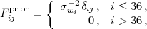
The weak dependence of w(z) constraints on the maximum SN redshift extends to other parameters as well. Figure 34 compares the effect on 1σ errors of varying the maximum SN redshift to that of varying the maximum BAO redshift. For the w0 - wa model, the errors on all parameters are relatively insensitive to changes in the maximum SN redshift at z ≳ 1, but the errors on wa and Ωk decrease by a factor of a few as the maximum BAO redshift increases from z = 1 to z = 3. Likewise, the high redshift equation of state w(z > 1) can be determined much more precisely as BAO data extend to higher redshifts, but it depends little on the maximum SN redshift. For the fiducial Stage IV forecasts, only the Hubble constant error depends significantly on the depth of SN observations (assuming a w0 - wa model). More pessimistic assumptions about the achievable BAO errors enhance the importance of high redshift SNe for determining wp (dotted line in Figure 34), but the dependence of other parameters on zmax for the SN data remains weak.
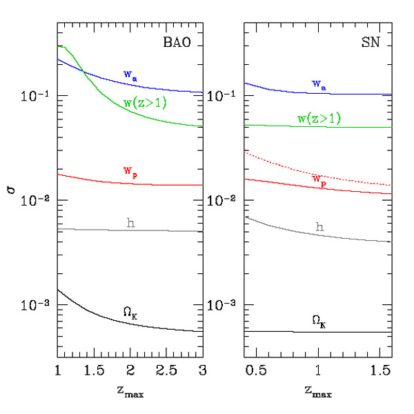 |
Figure 34. Variation of 1σ parameter errors with the maximum redshift for BAO at fixed fsky (left) or for SN with fixed error per Δz = 0.2 redshift bin (right). For the solid curves, fiducial Stage IV forecasts are assumed for all other probes. The dotted curve in the right panel shows the scaling of σ(wp) with SN zmax assuming 4 times larger BAO errors (BAO × 4). The plotted errors assume a w0 - wa parameterization (except for w(z > 1)). |
In practice, the impact of the maximum SN redshift on dark energy constraints will depend crucially on the behavior of systematic errors. We have assumed in our forecasts here that the error per redshift bin stays constant as the maximum SN redshift increases, but in reality higher redshift SNe are likely to have larger systematic errors associated with them, which would diminish the gains from high redshift SNe even more than indicated by the flattening of curves in Figure 33. However, once the systematic errors at z < 0.8 are saturated, then pushing to higher redshift may be the only way to continue improving the SN constraints. The gain from the higher redshift SNe then depends on whether their systematics are uncorrelated with those at lower redshift, so that they indeed provide new information. While there has been considerable recent progress in understanding and accounting of systematic errors in SN cosmology, there has been little exploration to date of the correlation of systematics across redshift bins. The correlation of systematics may vary with details of experimental design (e.g., flux calibration), and it also depends on aspects of the Type Ia supernova population that are, as yet, poorly understood (e.g., whether there is a mix of single-degenerate and double-degenerate progenitors that changes with redshift). To optimize a specific experiment, one must assess both the expected behavior of systematics and the observing time required to discover SNe at different redshifts and to measure them with adequate photometric and spectroscopic precision. The SDT report for WFIRST (Green et al. 2012) provides a worked example: with a two-tier strategy (shallow wide fields and narrow deep fields), the CMB+SN FoM increases steadily as the maximum redshift is increased from 0.8 to 1.7 at (roughly) fixed observing time, assuming systematics that are uncorrelated among redshift bins. However, reducing the systematics by a factor of two (from ≈ 0.02 mag per Δz = 0.1 bin to ≈ 0.01 mag) has a larger impact than raising zmax from 0.8 to 1.7. The contrast is less stark than in our Figure 33 because the reduction in total error is less than a factor of two; with the smaller systematic errors, the WFIRST DRM1 SN survey would be mainly statistics limited.
The behavior in Figure 33 can be approximately understood in terms of the aggregate measurement precision, a notion we discuss at greater length in Section 8.6 below. The local (z = 0.05) SN bin serves mainly to calibrate the SN absolute magnitude, so in our fiducial program there are three Δz = 0.2 redshift bins with cosmological information. Increasing zmax to 1.6 changes the number of non-local bins from three to seven, improving aggregate precision by ~ √7/3, and the impact on the FoM is roughly half the impact of reducing errors by a factor of two while retaining zmax = 0.8. If we increase zmax to 1.6 but simultaneously inflate the errors of the non-local bins by √7/3, thus keeping the aggregate precision of the z > 0.1 measurements fixed, then the FoM rises to 749, a 13% improvement over the fiducial case, vs. a 26% improvement if we increase zmax to 1.6 at constant per-bin error. In this sense, roughly half of the improvement when extending the redshift limit comes from tightening the aggregate statistical precision by adding new bins, and half the improvement comes from the greater leverage afforded by a wider redshift range. A similar calculation for zmax = 1.2 (where the corresponding FoM improvements over the fiducial case are 9% and 17%) leads to the same conclusion. Ultimately, however, the trade between extending the redshift range of a SN survey vs. improving the observations at lower redshift depends on aspects of observational and evolutionary systematics that are still poorly understood. This remains an important issue for near-term investigation with the much more comprehensive data sets that are now becoming available.
8.3.2. Constraints on structure growth parameters
While the DETF FoM is a useful metric for studying the impact of variations in each of the dark energy probes, it does not tell the whole story. Deviations from the standard model might show up in other sectors of the parameter space; for example, a detection of non-GR values for the growth parameters Δγ and G9 could point to a modified gravity explanation for cosmic acceleration that would not be evident from measurements of w(z) alone. Thus, even the less optimistic version of the WL experiment, which adds relatively little to the w(z) constraints obtained by the combination of fiducial SN, BAO, and CMB forecasts, is a critical component of a program to study cosmic acceleration because of its unique role in determining the growth parameters Δγ and G9.
The impact of various experiments on the structure growth parameters is more evident if we extend the DETF FoM to include Δγ in addition to w0 and wa. As shown in Figure 35, the scaling of this new FoM with respect to WL errors (and, to a lesser extent, BAO errors) is much steeper than it is for the usual FoM (Figure 33). We do not show the scaling with SN errors or zmax, since those assumptions do not affect the expected uncertainties for Δγ and G9 (see Table 8, lines 3-12). One could also consider versions of the FoM that include uncertainties in G9 and that account for the correlations between the structure growth parameters and the dark energy equation of state.
 |
Figure 35. FoM scaling with BAO errors (left) and WL errors (right) including changes in the error on Δγ, normalized to the forecast uncertainty for the fiducial program, σΔγfid = 0.034. The fiducial Stage IV forecast is marked by an open circle. For the Stage III forecast, FoMW (σΔγfid/ σΔγ) = 30. |
The complementarity between the SN, BAO, and WL techniques is further demonstrated in Figures 36 - 38, which show the forecast 68% confidence level contours in the w0.5 - wa and Δγ - lnG9 planes after marginalizing over other parameters. Instead of w0 we plot w0.5, the equation-of-state parameter at z = 0.5, because it is much less correlated with wa for most of the forecast scenarios. In every panel, the blue ellipse shows the error contour of the fiducial forecast while other ellipses show the effect of varying the errors of the indicated method. The opposite orientation of ellipses in Figures 36 and 37 demonstrates the complementary sensitivity of SN and BAO to w(z): the SN data are mainly sensitive to the equation of state at low redshift, whereas BAO data measure the equation of state at higher redshift. However, the sensitivity to the beyond-GR growth parameters comes entirely from WL data, which provide the only direct measurements of growth, and the strength of the Δγ and G9 constraints depends directly on the WL errors, as shown in Figure 38. Conversely, these constraints are very weakly sensitive to the SN or BAO errors (Figs. 36 and 37), showing that the uncertainties are dominated by the growth measurements themselves rather than residual uncertainty in the expansion history. Inspection of Table 8 shows that the Δγ constraints are essentially linear in the WL errors, while the lnG9 constraints scale more slowly.
 |
Figure 36. Forecast constraints (68% confidence levels) for dark energy and growth parameters, varying errors on SN data: fiducial × 4 (red), × 2 (green), W × (blue), and /2 (black). In all cases, the fiducial forecasts are used for the other probes (BAO, WL, CMB). Contours in the left panel use the value of the equation of state at z = 0.5 (close to the typical pivot redshift), w0.5 = w0 + wa/3. Dashed contours in the right panel show the errors on growth parameters for the binned w(z) parameterization, with the default priors corresponding to deviations of ≲ 10 in the average value of w. Solid contours assume a w0-wa parameterization. In both cases, the G9 and Δγ constraints are essentially independent of the SN errors. |
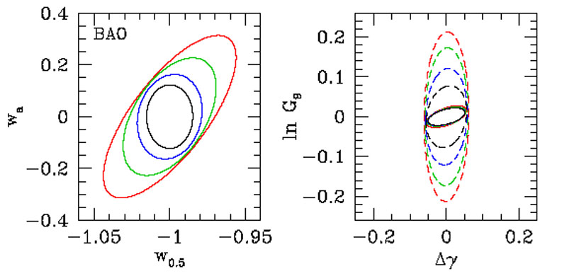 |
Figure 37. Same as Fig. 36, but varying BAO errors from fiducial × 4 (red) to fiducial/2 (black). |
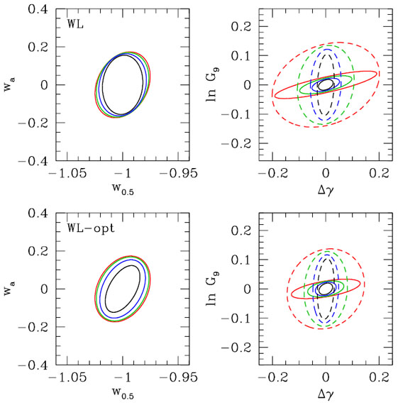 |
Figure 38. Same as Fig. 36, but varying WL errors from fiducial × 4 (red) to fiducial/2 (black). Lower panels assume the optimistic WL forecasts. |
Although the w0 - wa parameterization is flexible enough to describe a wide variety of expansion histories, it is too simple to account for all possibilities; in particular, w(z) is restricted to functions that are smooth and monotonic over the entire history of the universe. Because many cosmological parameters are partially degenerate with the dark energy evolution, assumptions about the functional form of w(z) can strongly affect the precision of constraints on other parameters. As an example of this model dependence, the right panels of Figures 36 - 38 show how the constraints on the growth parameters weaken (dashed curves) if one allows the 36 binned wi values to vary independently instead of assuming that they conform to the w0 - wa model. While Δγ forecasts are only mildly affected by the choice of dark energy modeling, constraints on the z = 9 normalization parameter G9 depend strongly on the form of w(z). This dependence follows from the absence of data probing redshifts 3 ≲ z < 9 in the fiducial Stage IV program. In the w0 - wa model, dark energy evolution is well determined even at high redshifts, since the two parameters of the model can be measured from data at z < 3, and thus the growth function at z = 9 is closely tied to the low redshift growth of structure measured by WL. However, allowing w(z) to vary independently at high redshift where it is unconstrained by data decouples the low and high redshift growth histories, and therefore G9 can no longer be determined precisely. In fact, the constraints on G9 in that case depend greatly on the chosen prior on wi (taken to be the default prior of σwi = 10 / √Δa in Figures 36 - 38). One important consequence of this dependence on the w(z) model is that an apparent breakdown of GR via G9 ≠ 1 might instead be a sign that the chosen dark energy parameterization is too restrictive.
8.3.3. Dependence on w(z) model and binning of data
Other parameters are also affected to varying degrees by the choice of w(z) model and the priors on the model parameters. Figure 39 shows how errors on Ωk and h are affected by relaxing assumptions about dark energy evolution. For the fiducial program and minor variants, Ωk is very weakly correlated with w0 and wa, resulting in similar errors on curvature for the w0 - wa and ΛCDM models. However, generalizing the dark energy parameterization to include independent variations in 36 redshift bins can degrade the precision of Ωk measurements by an order of magnitude or more. In that case, the error on Ωk is very sensitive to the chosen prior on the value of wi in each bin, and it improves little as the BAO errors decrease. This dependence on priors reflects the fact that curvature is most correlated with the highest redshift wi values, which are poorly constrained by the fiducial combination of data. Relative to curvature, constraints on the Hubble constant are affected more by the choice of dark energy parameterization but less by priors on wi in the binned w(z) model.
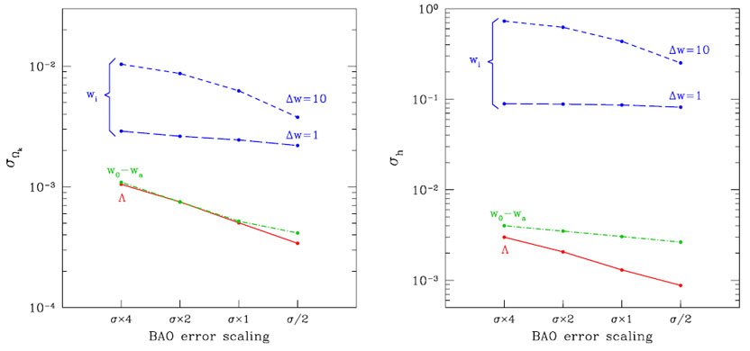 |
Figure 39. Dependence of σΩk (left) and σh (right) on BAO errors for various dark energy parameterizations and priors. For the wi curves, the equation of state varies independently in 36 bins with Gaussian priors of width σwi = Δw / √Δa. The fiducial versions of the Stage IV SN, WL, and CMB data are included in all cases. |
Figure 40 shows the dependence of σh on the precision of SN data for various dark energy parameterizations (σΩk is nearly independent of the SN errors for this range of variations around the fiducial forecast; see Table 8). If we assume a w0 - wa model for dark energy, Hubble constant errors strongly depend on the precision of SN data. However, Fig. 40 shows that either decreasing or increasing the number of dark energy parameters can almost completely eliminate the dependence of σh on the SN data. In the case of the simpler ΛCDM model, the combination of the fiducial BAO, WL, and CMB forecasts is sufficient to precisely determine all of the model parameters, and adding information from SN data has a negligible effect on the parameter errors. Adding w0 and wa to the model introduces degeneracies between these dark energy parameters and other parameters, including h. Since constraints from SN data help to break these degeneracies, reducing SN errors can significantly improve measurement of the Hubble constant in the w0 - wa model.
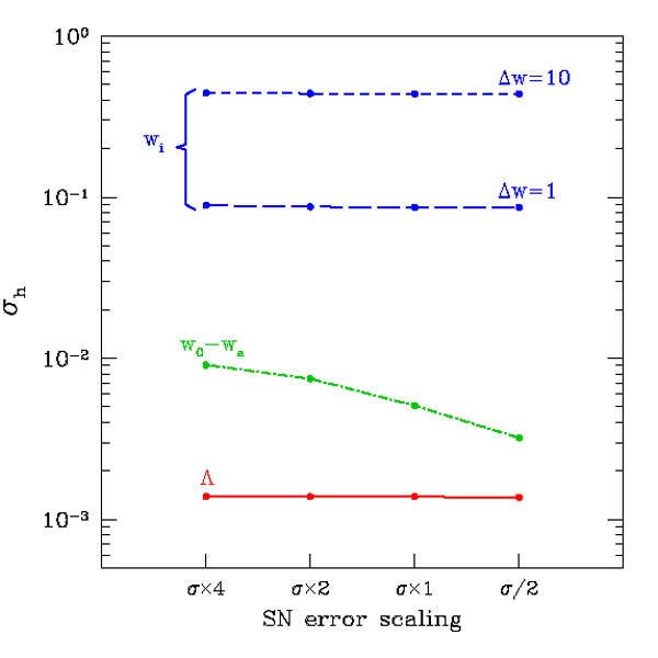 |
Figure 40. Dependence of σh on SN errors for various dark energy parameterizations and priors, including the fiducial BAO, WL, and CMB forecasts. |
As one continues to add more dark energy parameters to the model, the degeneracies between these parameters and h increase, but another effect arises that diminishes the impact of SN data on σh. Measurement of the Hubble constant requires relating observed quantities at z > 0 (e.g. SN distances) to the expansion rate at z = 0. In the case of ΛCDM or the w0 - wa model, the assumed dark energy evolution is simple enough that this relation between z = 0 and low-redshift observations is largely set by the model. However, when we specify w(z) by a large number of independent bins in redshift, this relation must instead be determined by the data. Since SN data are only sensitive to relative changes in distances, the lowest-redshift wi value (centered at z ≈ 0.01) is strongly degenerate with h (Mortonson et al. 2009a). This degeneracy is partially broken by the local SN sample at z = 0.05: removing it from the forecasts increases the error on h from 0.44 to 0.48 in the binned w(z) parameterization, and from 0.0051 to 0.0085 in the w0 - wa model. SNe at even lower redshifts are more sensitive to the Hubble constant, but they also have larger systematic uncertainties due to peculiar velocities.
For BAO data, the choice of redshift bin width affects forecasts for models with general equation-of-state variations. Measurements of H(z) and D(z) in narrower bins are better able to constrain rapid changes in w(z). They can also reduce uncertainty in the Hubble constant by about a factor of two, and in other parameters such as Ωk, lnG9, and Δγ by a smaller amount, relative to measurements in wide bins. However, in practice one cannot reduce the bin size indefinitely, since each bin must contain enough objects to be able to robustly identify and locate the BAO peak; for example, requiring that the bin be at least wide enough to contain pairs of objects separated by ~ 100 h-1 Mpc along the line of sight sets a lower limit of Δz / (1 + z) ≳ 0.03. We do not attempt to optimize the choice of bins for the simplified forecasts in this section, but we note that binning schemes in analyses of BAO data aimed at constraining general w(z) variations should be chosen with care to avoid losing information about dark energy evolution and other parameters. Similar concerns are likely to apply for WL data as well.
8.3.4. Constraints on w(z) in the general model
So far, in the context of general dark energy evolution we have only considered the forecast errors on parameters such as h and Ωk that are partially degenerate with w(z). But how accurately can w(z) itself be measured when we do not restrict it to specific functional forms? Since the errors on wi values in different bins are typically strongly correlated with each other, it is not very useful to simply give the expected wi errors, marginalized over all other parameters. Instead, we can consider combinations of the wi that are independent of one another and ask how well each of these combinations can be measured by the fiducial program of observations.
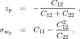
As mentioned in Section 2.2, many methods for combining w(z) bins into independent (or nearly independent) components have been proposed. Here we adopt the principal component (PC) decomposition of the dark energy equation of state. Starting from the Fisher matrix for the combined acceleration probes, the PCs are computed by first marginalizing the Fisher matrix over everything except for the wi parameters and then diagonalizing the remaining matrix, as described above in Section 8.2. The shapes of the three best-measured PCs for the fiducial program (with both fiducial and optimistic WL assumptions) and some simple variations are plotted in Figure 41. In general, the structure of the PCs is similar in all cases; for example, the combination of wi that is most tightly constrained is typically a single, broad peak at z < 1, while the next best-determined combination is the difference between w(z ~ 0.1) and w(z ~ 1). However, variations in the forecast assumptions slightly alter the shape of each PC and, in particular, shift the redshifts at which features in the PC shapes appear. Changes in the location of the peak in the first PC mirror the dependence of the pivot redshift zp for the w0 - wa model in Tables 8 - 10, with improved SN data decreasing the peak redshift and improved BAO data increasing it. The direction and magnitude of these shifts reflects the redshift range that a particular probe is most sensitive to and the degree to which that probe contributes to the total constraints on w(z). Note that so far we have only considered the impact of forecast assumptions on the functional form of PCs, and not on the precision with which each PC can be measured. In general, altering the forecast model changes both the PC shapes and PC errors, which complicates the comparison among expected PC constraints from different sets of forecasts.
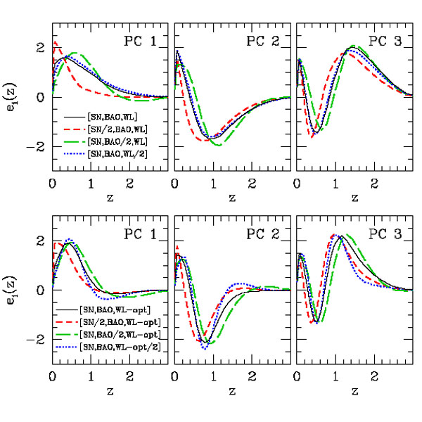 |
Figure 41. The three best-measured PCs for the fiducial program (solid curves) and from programs with SN, BAO, or WL errors halved (as labeled). The top row uses the fiducial version of the WL forecast, while the bottom row uses the optimistic WL forecast with reduced systematic errors. Although not indicated in the plot legends, all forecasts here include the default Planck CMB Fisher matrix. For all PCs shown here, ei(z) is nearly zero for 3 < z < 9. |
Comparing the top and bottom rows of panels in Figure 41, we see again the contrast between the fiducial WL forecast and the "WL-opt" forecast with reduced systematic errors. In the former case, decreasing WL errors by a factor of two has a negligible effect on the PC shapes relative to similar reductions in SN or BAO errors. However, when we take WL-opt as the baseline forecast the PCs depend more on the precision of WL measurements and less on that of the SN or BAO data.
| i | σifid | σiopt | i | σifid | σiopt | i | σifid | σiopt | i | σifid | σiopt |
| 1 | 0.011 | 0.009 | 10 | 0.135 | 0.102 | 19 | 0.442 | 0.378 | 28 | 1.652 | 1.810 |
| 2 | 0.017 | 0.014 | 11 | 0.143 | 0.116 | 20 | 0.779 | 0.413 | 29 | 2.285 | 2.217 |
| 3 | 0.026 | 0.019 | 12 | 0.168 | 0.137 | 21 | 0.824 | 0.436 | 30 | 3.243 | 2.973 |
| 4 | 0.038 | 0.026 | 13 | 0.180 | 0.150 | 22 | 0.939 | 0.531 | 31 | 6.540 | 6.785 |
| 5 | 0.052 | 0.036 | 14 | 0.185 | 0.160 | 23 | 0.978 | 0.609 | 32 | 12.43 | 19.20 |
| 6 | 0.067 | 0.047 | 15 | 0.216 | 0.179 | 24 | 1.212 | 0.725 | 33 | 16.59 | 24.78 |
| 7 | 0.083 | 0.062 | 16 | 0.252 | 0.240 | 25 | 1.307 | 0.892 | 34 | 25.17 | 46.41 |
| 8 | 0.099 | 0.074 | 17 | 0.310 | 0.244 | 26 | 1.457 | 1.036 | 35 | 59.32 | 94.09 |
| 9 | 0.115 | 0.089 | 18 | 0.323 | 0.308 | 27 | 1.587 | 1.561 | 36 | 74.12 | 118.0 |
| Note. — σifid refers to errors for the fiducial Stage IV program (CMB+SN+BAO+WL) and σiopt to the optimistic WL case (CMB+SN+BAO+WL-opt). | |||||||||||
The full set of PCs for the fiducial program is shown in Figure 42, and the forecast errors on the PC amplitudes are listed in Table 11. The best-measured, lowest-variance PCs vary smoothly with redshift, corresponding to averaging w(z) over fairly broad ranges in z. There is a clear trend of increasingly high frequency oscillations for higher PCs. Visual inspection of Figure 42 shows that the sum of the number of peaks and the number of troughs in the PC is equal to the index of the PC, a pattern that continues at least up to PC 13. Higher PCs often change sign between adjacent z bins. High frequency oscillations in w(z) are poorly measured by any combination of cosmological data because the evolution of the dark energy density, which determines H(z), depends on an integral of w(z) (eq. 22), and D(z) and G(z) depend (approximately) on integrals of H(z). Rapid oscillations in w(z) tend to cancel out in these integrals. Many of the most poorly-measured PCs depend on the chosen BAO binning scheme, since narrower BAO bins can better sample rapid changes in w(z). As an example, we show how the PCs of the fiducial program are affected by doubling the number of BAO bins in Figure 42.
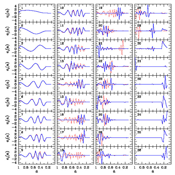 |
Figure 42. PCs for the fiducial program (solid blue curves). Dotted red curves double the number of bins used for BAO data from the default choice of 20 to 40. |
The maximum redshift probed by SN, BAO, and WL data, primarily set by the highest-redshift BAO constraint at z = 3 in our forecasts, imprints a clear signature in the set of PCs in Figure 42. At high redshift, specifically z > 3 (a < 0.25), the first 29 PCs have almost no weight. Conversely, PCs 30 and 32-36 only vary significantly at high redshift and are nearly flat for z < 3; additionally, the errors on these PCs are many times larger than those of the first 29 PCs. 77 Thus, w(z) variations above and below z = 3 are almost completely decoupled from each other in the fiducial forecasts, and the high-redshift variations are effectively unconstrained. CMB data limit the equation of state at z>3 to some extent, for example, through comparison of the measured distance to the last scattering surface with the distance to z = 3 measured in BAO data. However, such constraints are very weak when split among several independent w(z) bins at high redshift. Furthermore, since the dark energy density typically falls rapidly with increasing redshift, variations in w(z) at high redshift are intrinsically less able to affect observable quantities than low-redshift variations, resulting in reduced sensitivity to the high-redshift equation of state even in the presence of strong constraints at earlier epochs. Likewise, variations in w(z) at even higher redshifts of z > 9, where we assume that w is fixed to -1, are unlikely to significantly affect constraints on w(z) at low redshift. 78
Figure 43 shows how the inverse variance σi-2 of the 10 best-measured w(z) PCs increases relative to the fiducial program if we halve the errors on the SN, BAO, or WL data. Following Albrecht et al. (2009), when computing these ratios σ(2)i-2 / σ(1)i-2 (where 1 denotes the fiducial program and 2 the improved program), we first limit PC variances to unity by making the substitution σi-2 → 1 + σi-2, so that uninteresting improvements in the most poorly-measured PCs do not count in favor of a particular forecast. We caution that, as noted earlier, the PC shapes themselves are changing as we change the errors assumed in the forecast, so σ(2)i2 and σ(1)i2 are not variances of identical w(z) components. However, as shown in Figure 41, these changes are not drastic if we consider factor-of-two variations about our fiducial program.
The differences in σi-2 ratios among improvements in SN, BAO, and WL errors is striking. Relative to the fiducial program, reduced SN errors mainly contribute to knowledge of the first few PCs. For the fiducial WL systematics, reducing WL errors helps to better measure several of the highest-variance PCs in the plot (i > 10), but it makes little difference to the well measured PCs. Reducing BAO errors tightens constraints on nearly all of the PCs, with the greatest impact in the intermediate range between the SN and WL contributions. Assuming the optimistic WL errors gives much greater weight to WL improvements, which now produce the largest improvement in the first five PCs (right panel of Figure 43). The trends for reducing SN or BAO errors are similar to before, but the magnitude of their effect is smaller because they are competing with tighter WL constraints. The behavior of the σi-2 ratios of the best-measured PCs mirrors that shown for the DETF FoM in Figure 33. With the fiducial WL systematics, BAO measurements have the greatest leverage, followed by SN, and the impact of reducing WL errors is small. With the optimistic WL systematics, on the other hand, reducing WL errors makes the largest difference, followed by BAO, followed by SN.
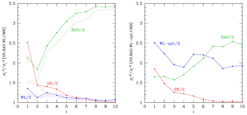 |
Figure 43. Ratios of inverse variances of PC amplitudes for variants of the fiducial program to the fiducial inverse variances (points and solid curves). Each variant divides SN, BAO, or WL errors by a factor of 2 while keeping other probes fixed at the fiducial errors. The left panel assumes the default WL forecast and the right panel assumes the optimistic version. Dotted curves in the left panel use σi instead of σi, which describes how well the amplitudes of the fiducial set of PCs are expected to be measured by some variant of the fiducial forecast. |
Dotted curves in the left hand panel show the σi-2 ratios when we fix the PCs to be those of the fiducial program. In this case, the PC errors for the improved programs are no longer uncorrelated, but the correlation coefficient of errors among any pair of PCs is less than 0.5 in nearly all cases. Results are similar to before except for the first component (first two components for BAO). These, of course, show less improvement when they are fixed to be those of the fiducial program rather than shifting to be the components best determined by the improved data. Figure 44 shows the expected improvements in σi-2 between our fiducial Stage III and Stage IV programs. Consistent with the DETF FoM plots in Figure 33, the expected improvements are dramatic, and considerably more so with the optimistic WL assumptions.
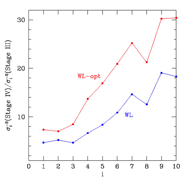 |
Figure 44. Ratios of inverse variances of PC amplitudes of Stage IV to those of Stage III, assuming either the fiducial or optimistic versions of the Stage IV WL forecast. |
The DETF FoM compresses constraints in the w0 - wa model to a single number. Similar figures of merit for PC constraints have been defined in the literature, in various forms, each of which may be useful for different purposes. These include the determinant of Fw, which characterizes the total volume of parameter space allowed by a particular combination of experiments in analogy to the DETF FoM for the w0 - wa parameter space, and the sum of the inverse variances of the PCs, which is typically less sensitive than the determinant to changes in the errors of the most weakly constrained PCs (Huterer and Turner 2001, Bassett 2005, Albrecht et al. 2006, Albrecht and Bernstein 2007, Wang 2008, Barnard et al. 2008, Albrecht et al. 2009, Crittenden et al. 2009, Amara and Kitching 2011, Mortonson et al. 2010, Shapiro et al. 2010, Trotta et al. 2011, March et al. 2011).
Examples of these FoMs for the fiducial program and the variants considered in Figure 43 are listed in Table 12. Here we allow the PC basis to change with the forecast assumptions, so Fw is diagonal and detFw = Πi = 136 σi-2. As with the ratios of PC variances in Figure 43, we restrict the variances to be less than unity by replacing σi-2 → 1 + σi-2. The other FoM, computed as the sum of inverse variances, requires no such prior because PCs with large variances contribute negligibly to the sum. Note that the choice of PC FoM definition can affect decisions about whether one experiment or another is optimal; for example, halving WL errors (assuming fiducial systematics) relative to the fiducial model increases the detFw FoM more than halving SN errors, but the opposite is true for the sum of inverse variances, which favors improvements in the best-measured PCs and more closely tracks the DETF FoM. In this case, at least, we regard the latter measure as a better diagnostic, since the improvements for PCs that are poorly measured in any case seem unlikely to reveal departures from a cosmological constant or other simple dark energy models. Another virtue of Σσi-2 (the square of the quantity tabulated in Table 12) is its sensible scaling with measurement precision. If the error of all the individual cosmological measurements (e.g., DL values and WL power spectrum amplitude) is dropped by a factor of two, as expected if experiments are statistically limited and data volume is increased by a factor of four, then each σi will drop by a factor of two and Σσi-2 will go up by a factor of four, scaling with data volume just like the DETF FoM. For detFw, on the other hand, the FoM will go up by ≈ 2N, where N is the number of PCs that have σi significantly below one, so there is no obvious scaling with data volume.
| Forecast case | log10 Πi = 136 (1 + σi-2)1/2 | (Σi = 136 σi-2)1/2 | [σ(wp) σ(wa)]-1 |
| [SN,BAO,WL,CMB] | 20.2 | 124 | 664 |
| [SN/2,BAO,WL,CMB] | 20.8 | 176 | 1197 |
| [SN,BAO/2,WL,CMB] | 26.0 | 186 | 1222 |
| [SN,BAO,WL/2,CMB] | 21.6 | 140 | 816 |
| [SN,BAO,WL-opt,CMB] | 23.0 | 157 | 789 |
| [SN/2,BAO,WL-opt,CMB] | 23.4 | 199 | 1242 |
| [SN,BAO/2,WL-opt,CMB] | 27.9 | 205 | 1251 |
| [SN,BAO,WL-opt/2,CMB] | 26.0 | 240 | 1397 |
The disagreement between different PC FoMs in Table 12 highlights one of the difficulties with using PCs or related methods for evaluating the potential impact of future experiments. Forecasts for PCs provide a wealth of information in both the redshift-dependent shapes of the PCs and the expected errors on their amplitudes, but it is often difficult to interpret what this information implies about cosmic acceleration. Given a set of forecasts for PCs, one can easily compute the expected constraints on any specific model for w(z) by expressing the model in terms of the PC amplitudes (eq. 174); this is a potentially useful application, but it makes very limited use of the available information.
More generally, we can use the forecast PC shapes and errors to try to visualize what types of w(z) variations are allowed by a certain combination of experiments. One approach is to generate several random w(z) curves that would be consistent with the forecast measurements. This method is easily implemented with the PCs because the errors on different PC amplitudes are uncorrelated. One can generate a random realization of w(z) by simply drawing an amplitude αi from a Gaussian distribution with mean zero and width σi, then using equation (175) to compute w(z) corresponding to the randomly-drawn αi values.
In the upper left panel of Figure 45, we use this method to plot several w(z) models using the fiducial program PC shapes and errors from Figure 42 and Table 11, respectively. We cut off the plot at z = 3, since w(z) variations at higher redshifts are essentially unconstrained by the fiducial experiments. Even at lower redshifts, though, the allowed w(z) variations are enormous, with wi values often changing by 10 or more from one bin to the next. (Recall that our prior corresponds to a Gaussian of width σwi ≈ 63 per bin, eq. 172.) Compared to the ~ 1.5% constraints on wp in the w0 - wa model, this forecast looks rather depressing. The consequence of allowing the equation of state to be a free function of redshift is that it is nearly impossible to say with any certainty what the value of w is at any specific redshift, because rapid oscillations in w(z) have tiny effects on observables. The allowed range of variations would be even larger if we considered a model with finer Δa bins.
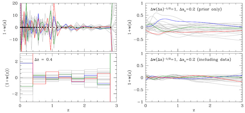 |
Figure 45. Reconstruction of w(z) from PC constraints. Left: 20 randomly-generated models that would be indistinguishable from a cosmological constant using the fiducial program of experiments. Three of the 20 models are highlighted (in red, green, and blue) to more clearly show examples of the evolution with redshift. The lower panel shows the average of 1 + w(z) in bins of width Δz = 0.4 for the same models as in the upper panel. Points along the w(z) = -1 line in the upper panel mark the centers of the bins in which w(z) is allowed to vary in our forecasts. Right: w(z) reconstruction including a prior of the form in equation (178). The upper panel shows a random selection of models consistent with this prior, but without including any data, and the lower panel shows examples of models that are allowed by both the prior and the data assumed in the fiducial program. |
The large variations of w(z) in Figure 45 are driven by the poorly constrained PCs, which have many oscillations in w(z), peak-to-peak amplitudes |Δw| ~ 4, and normalization uncertainties σi ~ 0.1-2.3 (see Figure 42 and Table 11). The lower left panel of Figure 45 shows these w(z) realizations averaged over bins of width Δz = 0.4, which vastly reduces the range of variations, especially at z ~ 1. However, the dispersion of w(z) in the bins centered at z = 0.6 and z = 1 is still about 0.3. Adding a precise, independent measurement of H0 reduces the uncertainty in w(z) in the lowest-redshift bin, but it has little effect at higher redshifts (see Section 8.5.1).
Instead of averaging w(z) over wide redshift bins, one can impose a theoretical prejudice for models with smoothly-varying equations of state by adding an off-diagonal prior to the Fisher matrix, imposing correlations among the wi that are closely separated in redshift. Here we follow Crittenden et al. (2009), but we modify their method to use scale factor rather than redshift as the independent variable (see also Crittenden et al. 2012), adopting a correlation function
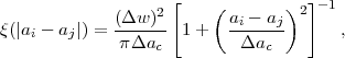 |
(177) |
where Δw sets the amplitude of allowed w(z) variations and Δac is the correlation length. Following the calculation in Crittenden et al. (2009), the covariance matrix for the wi bins, which is the inverse of the prior Fisher matrix for those parameters, is
 |
(178) |
where  = |i - j|
Δa /
Δac,
x+ = (|i - j| + 1)
Δa /
Δac, and x- = (|i -
j| - 1)
Δa /
Δac.
In the limit Δac
→ 0, this reduces to our default diagonal
prior on the wi parameters with width
σwi =
Δw /
√Δa.
= |i - j|
Δa /
Δac,
x+ = (|i - j| + 1)
Δa /
Δac, and x- = (|i -
j| - 1)
Δa /
Δac.
In the limit Δac
→ 0, this reduces to our default diagonal
prior on the wi parameters with width
σwi =
Δw /
√Δa.
The upper right panel of Figure 45 shows models randomly drawn from this prior with Δw / √Δa = 1 and Δac = 0.2. The influence of the correlation function is clearly evident in the smoother, lower-amplitude variations of w(z) in these models, and yet the range of possible models is still much greater than for simpler parameterizations like w0-wa. Combining this prior with the assumed data set of the fiducial Stage IV program, we obtain the w(z) realizations plotted in the lower right panel of Figure 45. Even more so than averaging w(z) in wide redshift bins, including this type of prior significantly narrows the constraints on w(z). While the particular smoothness prior of (177) is certainly not unique, this approach of combining PC constraints dictated by the data sets with theoretically motivated priors on the behavior of w(z) — perhaps based on an underlying model for the potential V(ϕ) — may be the most valuable application of the PC approach.
Our constraints on general w(z) models account for the possibility of modified gravity by marginalizing over the structure growth parameters Δγ and lnG9. If we instead restrict our analysis to GR by fixing Δγ = lnG9 = 0, the main effect is that the dark energy equation of state at high redshifts, w(3 < z < 9), is better constrained because the CMB measurement of the power spectrum amplitude at z ~ 1000 can be more directly related to WL measurements of growth at lower redshifts. Because of the additional CMB constraint on the distance to the last scattering surface, w(3 < z < 9) is strongly correlated with Ωk, and therefore assuming GR considerably improves the determination of spatial curvature in the binned w(z) parameterization. For our fiducial forecasts, assuming Δγ = lnG9 = 0 lowers σΩk by a factor of ~ 3 (0.0075 → 0.0023); note that this is still several times larger than the error in Ωk for the simpler ΛCDM or w0 - wa forecasts.
We have concentrated so far on the constraints expected for combinations of CMB, SN, BAO, and WL data, as all of these methods are well studied and are likely to play a central role in Stage III and Stage IV studies of cosmic acceleration. For other methods we adopt a simplified approach, first asking how well our fiducial CMB+SN+BAO+WL programs should predict the basic observables of these methods, then showing how different levels of precision on these observables would affect constraints on equation-of-state and growth parameters. We describe our methodology more fully in the next section (Section 8.5), but we begin with a discussion of clusters, where our analysis of stacked weak lensing calibration (Section 6.3.3) gives a clear quantitative target for measurement precision.
Figure 46a shows the predicted fractional error (1σ) in σ8(z) for the fiducial Stage III and Stage IV experimental programs discussed in Section 8.3, and for the Stage IV program with optimistic WL errors. All curves assume a w0 - wa dark energy parameterization, and for each case the lower, thinner curve shows the forecast assuming GR to be correct while the upper, bolder curve allows GR deviations parameterized by G9 and Δγ. Roughly speaking, we would expect a measurement with precision better than that shown by the upper curve to significantly improve tests for GR deviations and a measurement with precision better than that shown by the lower curve to significantly improve w0 - wa constraints when assuming GR to be correct. For Stage IV programs we predict σ8(z) constraints at the 0.75-1% level over the full redshift range 0 < z < 3, with little difference between the fiducial and optimistic WL assumptions. In fact, the "optimistic" WL assumptions lead to slightly larger errors in σ8(z) than the fiducial assumptions because for this quantity doubling the statistical errors has a larger impact than adding 2 × 10⁻³ shear calibration and photo-z errors (see Section 8.1). For Stage III, the predicted σ8(z) errors are about 1.2% assuming GR, but they are much larger if we allow GR deviations, especially at z > 0.8. Even for Stage IV, the good constraints at high z rely on the assumption of a w0 - wa equation of state, which allows precise low redshift WL measurements to be extrapolated to high redshift. The direct measurements of z > 1 clustering amplitude are considerably weaker.
 |
Figure 46. (a) Predicted fractional errors (1σ) on σ8(z) from our fiducial Stage III (dotted) and Stage IV (solid) CMB+SN+BAO+WL programs, and from the Stage IV program with optimistic WL systematic assumptions (dashed). All curves assume a w0 - wa dark energy parameterization. For each case, the lower, thin curve shows the forecast assuming GR is correct and the upper, thick curve shows the forecast allowing GR deviations parameterized by G9 and Δγ. (b) Like (a), but for σ11,abs(z), the rms matter fluctuation in spheres of radius 11 Mpc (instead of 8 h-1 Mpc). (c) Like (b), but for the parameter combination σ11,abs(z) Ωm0.4 that approximates the quantity best constrained by cluster abundances. (d) Predicted fractional errors in σ11,abs(z) Ωm0.4 from cluster abundances in a 104 deg2 survey calibrated by stacked weak lensing mass estimates with Stage III (neff = 10 arcmin-2) and Stage IV (neff = 30 arcmin-2) source surface densities and survey depths (dotted and solid curves, respectively). From top to bottom, curves correspond to cluster mass thresholds of 8, 4, 2, and 1 × 10¹⁴ M⊙. |
Figure 46b plots σ11,abs(z) errors, which are tighter than the σ8(z) errors by ~ 30-50% because uncertainty in h contributes noticeably to the latter. In Section 6.6 we estimated the errors on σ11,abs(z) achievable with a 104 deg2 cluster survey with weak lensing mass calibration, assuming Stage III (10 arcmin-2) or Stage IV (30 arcmin-2) effective source densities and survey depths. For a mass threshold of 2 × 10¹⁴ M⊙ the σ11,abs(z) errors at z ≈ 0.5 are ~ 1% and ~ 0.5%, respectively, below the corresponding Stage III and Stage IV errors shown in Figure 46b. Furthermore, these cluster errors are per Δz = 0.1 redshift bin, so constraints on the clustering amplitude in a smoothly evolving model can be substantially better if the cluster errors are not correlated across redshifts. (The statistical errors should be uncorrelated, but some forms of weak lensing systematics could affect many redshift bins in the same direction.)
The cluster errors shown earlier in Figure 30 were derived assuming perfect knowledge of Ωm, with σ11,abs(z) as the single parameter controlling the cluster abundance at each redshift. In practice, cluster abundances constrain a parameter combination that is approximately σ11,abs(z) Ωm0.4, as discussed in Section 6. The fractional errors in Ωm from our fiducial CMB+SN+BAO+WL programs are 2.7% (Stage III), 1.4% (Stage IV), and 1.2% (Stage IV with WL-opt), making Ωm0.4 uncertainties comparable to the fractional errors in σ11,abs(z). Figure 46c shows the predicted fractional errors in σ11,abs(z) Ωm0.4, which in some ranges are significantly larger than those for σ11,abs(z). Finally, Figure 46d shows our forecast errors on σ11,abs(z) Ωm0.4 from a 104 deg2 cluster survey in which errors are limited by weak lensing mass calibration statistics. Here we have simply set the fractional errors from clusters on σ11,abs(z) Ωm0.4 equal to the ones we derived earlier on σ11,abs(z), which should be a good but not perfect approximation. Comparing Figures 46c and 46d shows that cluster errors are competitive with those expected from the CMB+SN+BAO+WL combination for cluster mass thresholds of ~ 4-8 × 10¹⁴ M⊙ at Stage III or 1-4 × 10¹⁴ M⊙ at Stage IV.
Figure 47 shows the potential improvement in equation-of-state and growth parameter determinations from including the cluster constraints on σ11,abs(z) Ωm0.4. We assume that these constraints have independent errors in each Δz = 0.1 bin. Upper panels show the effect of adding Stage III cluster constraints (dotted curves in Fig. 46d) to the Stage III CMB+SN+BAO+WL Fisher matrix. Even adding clusters with an 8 × 10¹⁴ M⊙ mass threshold substantially improves the errors on G9 and Δγ, and reducing the mass threshold to 1-2 × 10¹⁴ M⊙ produces substantial further gains. Somewhat surprisingly, the cluster constraints also lead to significantly smaller errors on the equation-of-state parameter w0.5 and slightly smaller errors on wa. This improvement largely reflects the additional information about Ωm, which allows the distance and H(z) constraints from other probes to translate more directly into w(z) constraints. We have checked that fixing Ωm exactly would produce a still greater improvement in (w0.5, wa) than the gain we have forecast from clusters, while making little difference to the (G9, Δγ) errors.
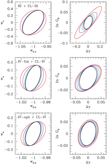 |
Figure 47. Predicted constraints (1σ) on the equation-of-state parameters w0.5 = w(z = 0.5) and wa (left panels) and the growth parameters G9 and Δγ (right panels) from our fiducial CMB+SN+BAO+WL programs combined with cluster abundance measurements of σ11,abs(z) Ωm0.4 with the precision shown in Fig. 46d. Top panels show Stage III clusters with Stage III CMB+SN+BAO+WL, while middle and bottom panels show Stage IV clusters combined with the fiducial and WL-opt Stage IV programs, respectively. Note the change in axis scale between the top and middle/lower panels. In each panel, the outermost contour shows the constraints without clusters, and the remaining contours show the constraints for cluster mass thresholds of 8, 4, 2, and 1 × 10¹⁴ M⊙ (outer to inner). |
For Stage IV (middle and bottom panels), where we now assume the Stage IV cluster mass constraints, an 8 × 10¹⁴ M⊙ cluster sample produces little improvement over CMB+SN+BAO+WL in G9 and Δγ, but it still leads to noticeable improvement in w0.5. A 1-2 × 10¹⁴ M⊙ cluster sample produces substantial gains in both the equation-of-state and growth parameters. As in the Stage III case, much of the improvement in the equation of state comes from the Ωm information provided by clusters. However, the cluster constraints reduce the w0.5 error even if Ωm is held fixed, so some of this improvement arises from another source, probably by allowing some WL information to be effectively transferred from growth to distance. Adding our Stage IV, 1014 M⊙ cluster constraint to the fiducial Stage IV program increases the DETF FoM from 664 to 1258, and it increases the modified FoM [σ(wp) σ(wa)]-1 × [0.034 / σ(Δγ)] (Figure 35) from 664 to 1955. For the WL-opt program, the improvements are 789 → 1363 and 1037 → 2380, respectively. For Stage III CMB+SN+BAO+WL, adding Stage III clusters leads to improvements of 131 → 183 (FoM) and 30 → 137 (modified FoM).
Our treatment here is simplified because we have ignored the impact of volume-element changes on the cluster abundance and have set the scaling index of σ11,abs(z) Ωmq to a constant value q = 0.4 instead of including its redshift and mass dependence. More importantly, we have assumed that errors in the cluster abundance will be dominated by the statistical errors in the weak lensing calibration of the mean mass scale, not increased by marginalizing over uncertainties in mass-observable scatter, incompleteness, contamination, or theoretical predictions. The effective mass calibration uncertanties we are assuming are those in Figure 28. These are probably pessimistic at z ≳ 1, where the weak lensing calibration error exceeds 10% but one could likely use other calibration methods (including direct comparison to theory) to do better; thus, we are underplaying the potential contribution of high-redshift clusters. Our approximate calculations confirm the conclusions of Oguri and Takada (2011) that clusters calibrated with stacked weak lensing can make an important contribution to testing cosmic acceleration models, even in the era of Stage IV dark energy experiments. Figure 46 also provides a target for other methods of measuring the matter clustering amplitude, such as the Lyα forest (Section 7.6).
8.5. Forecasts for Alternative Methods
We now turn to some of the alternative probes discussed previously in Section 7. For each technique, we first focus on the question of complementarity with the primary methods by asking how well the observable quantity measured by a particular technique is already known given the fiducial combination of SN, BAO, WL, and CMB data. These predictions provide benchmarks that any additional measurement must reach in order to contribute significantly to constraints on dark energy or modified gravity parameters. In many cases, the precision of the predictions depends strongly on the chosen parameterization of deviations from the standard paradigm of ΛCDM and GR. We will generally assume a w0 - wa model for the results in this section, but we note that if one adopts a more general parameterization of dark energy then the predictions are normally weaker, and thus the value of alternative probes is potentially greater.
The covariance matrix for a set of observables x measured by a particular alternative probe can be computed straightforwardly using the covariance matrix of the cosmological parameters given by the inverse of the total Fisher matrix for SN, BAO, WL, and CMB data,
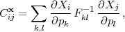 |
(179) |
where p is either the full set of parameters in eq. (162) or the reduced set with w0 and wa replacing the 36 wi bins; in the latter case, F is the Fisher matrix for the w0 - wa parameterization computed using eq. (170). We compute the full covariance matrices for the alternative methods, but the plots in the following sections only show the predicted uncertainties σXi = (Ciix)1/2 and do not reflect the fact that errors on the observables may be correlated.
In addition to computing how well the fiducial SN, BAO, WL, and CMB constraints predict each observable that would be measured by the alternative techniques, we provide several examples to show the improvement in the FoM and other parameters that would result from a specific measurement of that observable. For these tests, we only consider the impact of measurement of a single quantity X at a time, so the total Fisher matrix is modified simply by adding the term
 |
(180) |
where σX is the assumed uncertainty in the measurement of X.
For the Hubble constant, the predicted uncertainty from the fiducial probes is simply the value of σh that comes out of the Fisher matrix forecasts of the previous section. Assuming a w0 - wa dark energy model, the expected precision on H0 is 0.7% for the fiducial Stage IV forecasts and small variations of those forecasts, and 1.3% for Stage III (see Tables 8 - 10). These are challenging, but probably attainable, targets for future efforts to independently measure H0.
In Figure 48, we show the effect on the DETF FoM of adding a prior on H0 to the fiducial Stage III and IV forecasts. In all cases, adding a prior with precision that matches the uncertainty one would have in the absence of the prior increases the FoM by ~ 40%. The uncertainties in other cosmological parameters are affected little by the inclusion of an independent H0 measurement, as discussed in Section 7.1.
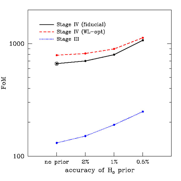 |
Figure 48. Dependence of the DETF FoM on the accuracy of additional measurements of the Hubble constant for Stage III and IV forecasts from Section 8.3. The fiducial Stage IV program with FoM=664 is marked by an open circle. |
For a more general dark energy parameterization such as the binned wi values, predictions for σh can be orders of magnitude weaker than they are for w0 - wa or ΛCDM (see Figs. 39 - 40). In this case an independent, local measurement of H0 is vital for accurate determination of the Hubble constant. However, H0 priors do not significantly improve dark energy constraints in this case; an H0 constraint limits the range of w(z) in the lowest-redshift bin, but since w(z = 0) is only weakly correlated with the equation of state at higher redshifts by SN, BAO, WL, and CMB data, the impact of an additional H0 measurement on the equation of state at z > 0 is small. The improvement in the DETF FoM in Fig. 48 is largely a consequence of the restrictions that the w0 - wa parameterization places on the evolution of w(z) between z = 0 and higher redshifts. Of course, a discrepancy between directly measured H0 and a w0 - wa prediction would already provide the crucial insight that w0 - wa is inadequate; it just wouldn't give further direction about the evolution of w(z).
8.5.2. The Alcock-Paczynski Test
For the AP test (Section 7.3), we consider the observable H(z) DA(z). Since Stage IV BAO data provide tight constraints on both H(z) and DA(z), which are further strengthened by the SN, WL, and CMB measurements, it is not surprising that the product H(z) DA(z) is predicted very precisely in the combined forecasts. The left panel of Figure 49 shows that the uncertainty in the AP observable is ~ 0.2% at 0< z < 3 for Stage IV data, and it is still predicted to sub-percent accuracy with Stage III data. Independent measurements of the AP observable that are significantly less precise than these predictions would contribute little to cosmological constraints. Note that these results are for a w0 - wa dark energy model. If we instead use independently-varying w(z) bins, the uncertainty in the AP observable for the Stage IV forecasts increases to ~ 1% at 1 < z < 3 and becomes much larger at both lower and higher redshifts, although the exact precision of the predictions in this case depends strongly on the detailed forecast assumptions such as the prior on wi in each bin or the number of bins used for BAO data.
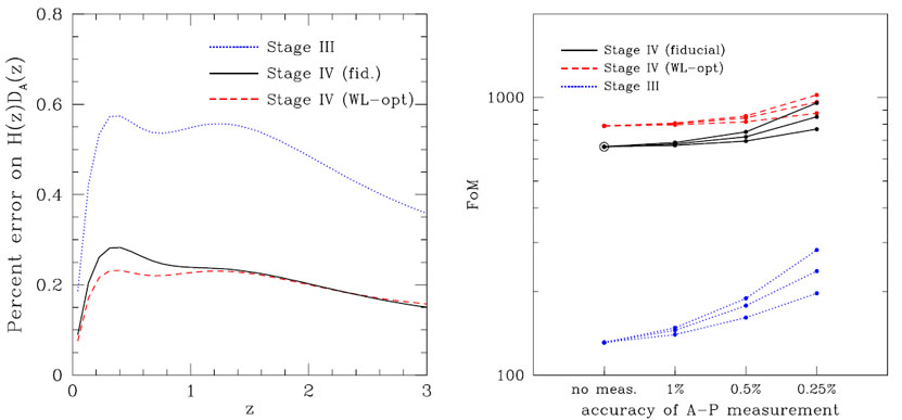 |
Figure 49. Left: Predicted fractional error (1σ) of the AP parameter H(z) DA(z) from our fiducial Stage III and Stage IV CMB+SN+BAO+WL programs, assuming a w0 - wa dark energy parameterization. Right: Dependence of the DETF FoM on additional measurements of H(z) DA(z) at a single redshift. For each forecast, the three curves from top to bottom assume AP measurements at z = 0.5, z = 1, and z = 2, respectively. |
In the right panel of Fig. 49, we show the improvement in the DETF FoM (assuming the w0 - wa parameterization) when various measurements of the AP observable are added to the fiducial Stage III and IV forecasts. Since the predictions for H(z) DA(z) are weakest at z ≲ 0.5, a direct measurement of the AP observable at those redshifts has a greater impact on the FoM than measurements at higher redshifts. 79 A 1% measurement of H(z) DA(z) at z = 0.5 increases the Stage III FoM by about 13%; a similar improvement in the Stage IV FoM requires an accuracy of 0.5% at the same redshift. While the demands suggested by Figure 49 appear stiff, large redshift surveys in principle have the information to achieve very high precision on H(z) DA(z). The challenge is lowering systematics to the level needed to achieve this precision.
8.5.3. Redshift-space Distortions
For redshift-space distortions (RSD; Section 7.2), the relevant observable is σ8(z) f(z). WL data provide some limits on this observable by constraining the structure growth parameters Δγ and (in combination with the CMB) G9, and through their constraints on the expansion history all of the acceleration probes contribute indirectly to the predicted growth history. The resulting predictions for Stage III and IV programs are plotted in the left panel of Figure 50. We show predictions both for the general case where we marginalize over the structure growth parameters and for GR (Δγ = lnG9 = 0).
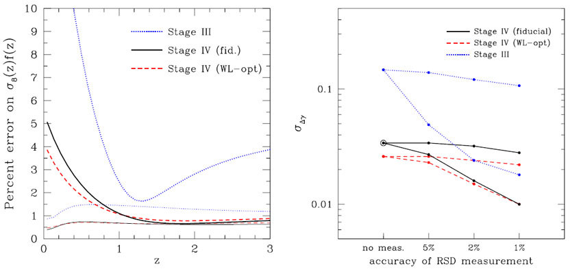 |
Figure 50. Left: Predicted fractional error (1σ) of the RSD observable σ8(z) f(z) from our fiducial Stage III and Stage IV CMB+SN+BAO+WL programs, assuming a w0 - wa dark energy parameterization. The lower, thin curves for each forecast additionally assume GR by fixing Δγ = lnG9 = 0. Right: Improvement in the 1σ uncertainty on Δγ from an additional RSD measurement at a single redshift. For each forecast, the lower and upper curves assume RSD measurements at z = 0.2 and z = 1, respectively. |
With the assumption of GR, the RSD observable is predicted to 1-2% accuracy for Stage III and 0.5-1% accuracy for Stage IV. If we allow modifications to GR through Δγ and G9, however, the uncertainty at z < 1 increases dramatically. This change is mainly tied to the freedom to alter the growth rate f(z) at low redshift by varying Δγ. Note that the effect of Δγ vanishes at high redshift because Ωm(z) approaches unity and therefore f(z) → fGR(z) (see equation 44). At z ≳ 2, uncertainty in G9 significantly weakens Stage III predictions of the RSD observable, but the effect on Stage IV predictions is much smaller.
The DETF FoM can be improved by the addition of precise RSD measurements if we assume GR; for example, the fiducial Stage IV (Stage III) FoM increases by ~ 10-15% with a 1% (2%) RSD constraint at z = 1. Without assuming GR, the additional information from an RSD measurement at a single redshift goes mainly into constraining the structure growth parameters (and thus testing GR). In this case, the FoM improvement from percent-level RSD constraints is ≲ 10%. However, percent-level measurements in several redshift bins can still have an important impact on the FoM.
Low-redshift measurements of the RSD observable can contribute significantly to constraints on Δγ, as shown in the right panel of Fig. 50. For Stage III forecasts, 1-2% RSD measurements at z = 0.2 reduce the error in Δγ by nearly an order of magnitude, reaching an uncertainty comparable to that expected from the Stage IV probes. Likewise, the Stage IV constraint on Δγ can be improved by a factor of a few by the addition of percent-level RSD measurements. At higher redshifts, the impact of RSD observations on the Δγ uncertainty is greatly reduced due to the diminishing effect of Δγ on the growth rate at high z. This reduced sensitivity at high z is in some sense an artifact of the Δγ parameterization; the error on Δγ is larger than the error on lnf by a factor |(dlnf / dΔγ)-1| = |[lnΩm(z)]-1|, which for the fiducial cosmological model of Table 7 is 1.02 at z = 0.2 [where Ωm(z) = 0.373] and 3.23 at z = 1 [where Ωm(z) = 0.734].
We have computed but not plotted the impact of RSD measurements on the growth normalization parameter G9. For Stage IV, the uncertainty in G9 is little affected by adding RSD measurements at any redshift. For Stage III, 1-2% measurements of σ8(z) f(z) can reduce the fractional error in G9 by up to a factor of two. As discussed in Section 7.7, some modified gravity theories predict a mismatch between measures of structure using non-relativistic tracers, which respond to the Newtonian potential Ψ (eq. 159), and measures based on weak lensing, which responds to Ψ + Φ, the sum of the Newtonian potential and space curvature. Consistency between RSD and WL, or cluster masses calibrated by weak lensing, tests for deviations of this sort, in addition to the G9 and Δγ constraints obtained by combining the measurements assuming Ψ = Φ.
As a target for alternative distance indicator methods (Section 7.4) and standard sirens (Section 7.5), Figure 51 plots the predicted fractional error on the angular diameter distance from our fiducial Stage III and Stage IV CMB+SN+BAO+WL programs. If we assume a w0 - wa model then the constraints are tight, better than ≈ 0.25% for Stage IV and ≈ 0.5% for Stage III at all z > 0.5. However, the highest redshift distance measurements included in our forecasts (other than CMB) are BAO measurements at z = 3, so when we change to our general w(z) model the distance errors at z > 4 become dramatically worse, ≈ 2% for Stage IV and ≈ 8% for Stage III. Furthermore, our Stage III forecast assumes a 0.8% distance measurement from HETDEX at z = 2.4, which we consider somewhat optimistic because it assumes that the full power spectrum shape can be used rather than the BAO scale alone. At z < 2 the Stage III curve has a jagged structure that depends to some degree on the specific choices we have made in binning and in assigning BAO/WL measurements to particular redshifts.
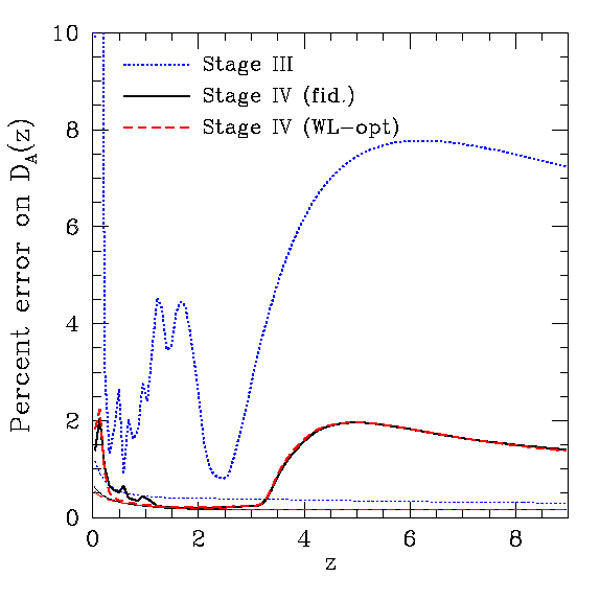 |
Figure 51. Predicted fractional error (1σ) on the distance DA(z) from our fiducial Stage III and Stage IV CMB+SN+BAO+WL programs and the Stage IV program with optimistic weak lensing assumptions. For each case, the lower, thin curve assumes a w0 - wa dark energy parameterization, while the upper, thick curve represents our binned w(z) model. |
The message to take away is that Stage III distance errors for the general w(z) model should be in the 1-2% range at z<1, the 3-5% range at 1 < z < 2, and the 6-8% range at z>4, with the errors at 2 < z < 4 depending on the strength of BAO measurements from Lyα emission line galaxies (HETDEX) or the Lyα forest (BOSS). On the Stage III timescale, alternative distance measurements at z>1 with few percent precision could reveal otherwise hidden departures from the w0 - wa model. For Stage IV, where we assume powerful BAO experiments extending to z = 3, the demands on alternative distance indicators are much stiffer. Even for the general w(z) model, alternative measures at z > 4 must reach 2% precision to be competitive. The Stage IV distance errors in this model become large at z < 0.25, similar to the several percent errors in H0 seen in Figure 40. As already discussed in Section 8.5.1, precise low redshift distance measurements have the potential to reveal late-time departures from smooth w(z) evolution.
8.6. Observables and Aggregate Precision
We have characterized the performance of the fiducial program and its variants in terms of their ability to constrain parameterized models, from the specific (w0 - wa + GR) to the general (w(zi), G9, Δγ). An alternative, more model-agnostic approach to characterizing the power of an experiment is via the aggregate precision with which it measures its basic observable. We have already introduced this idea at a few points, most notably in our discussion of BAO. By "aggregate precision" we mean the fractional (1σ) error on an overall factor that multiplies the observable in all redshift bins (and, if applicable, angular or mass bins). For the simple case of an observable O with independent fractional measurement errors ΔlnO(zi) in N redshift bins, the aggregate precision follows from the quadrature combination of the individual errors:
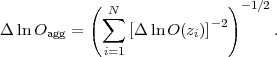 |
(181) |
One important virtue of forecasting an experiment's aggregate precision is that it focuses one's attention on the required control of systematics, especially systematics that are correlated across redshift bins.
Figure 52 plots the errors on the observables
in our fiducial SN, BAO, and WL programs. For SN (upper right),
we adopt independent errors of 0.01 mag in each of four redshift
bins, corresponding to fractional errors in luminosity distance
of 0.46%. The aggregate measurement precision is therefore
ΔlnDL,agg = 0.23%. This is equal to the
aggregate precision forecast for the SN component of the WFIRST
design reference mission (DRM1) forecast by
Green et al. 2012)
for their "optimistic" assumption about SN systematics.
80
However, the measurement in the z = 0.05 bin goes mainly
to constraining the nuisance parameter
, the
SN absolute magnitude scale, so it is arguably better to characterize
our fiducial program's aggregate precision as 0.46% /
√3 = 0.27%,
which is closer to that of the "conservative" WFIRST
forecast (0.32%).
More generally, we note that large local calibrator samples are
likely to achieve high statistical precision, and the systematic
uncertainty in relating this local sample to fainter, redshifted
samples will play a crucial role in determining the cosmological
performance of the SN program.
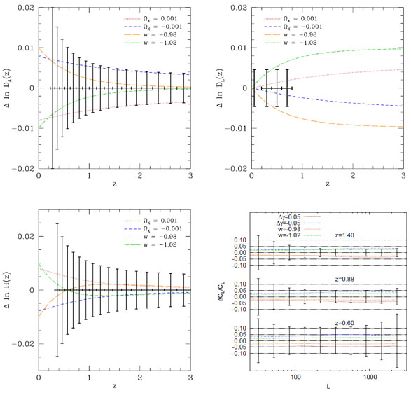 |
Figure 52. Forecast errors for fiducial
Stage IV SN, BAO, and WL programs, compared to model deviations from
fiducial
ΛCDM.
The top panels show the forecast fractional errors in
angular diameter distance from BAO (left) and luminosity
distance from SNe (right), in absolute (Mpc) and relative
(h-1 Mpc) units, respectively.
The lower left panel shows the H(z) error from BAO.
The errors are uncorrelated from bin to bin,
though the DA(z) and H(z) errors
in each bin are correlated with each other.
Curves show the fractional changes in the predicted relations relative to
the fiducial cosmology for CMB-normalized models with
1 + w = ± 0.02 or
Ωk = ± 0.001, as labeled.
Marginalization over
|
The left panels show the fractional errors predicted on DA(z) and H(z) for the fiducial BAO program, as tabulated in Table 6. These error bars decrease with increasing redshift because of the greater comoving volume per Δln(1 + z) bin at high redshift. Comparison of the DL and DA panels nicely illustrates the complementarity of SN and BAO as low and high redshift probes, respectively, though recall that they provide distinct information even at the same redshift because of relative vs. absolute calibration. The aggregate precision of the BAO measurement is ΔlnDA,agg = 0.13%, tighter than that from SNe because of the larger number of bins. Statistical errors in H(z) are larger by a factor of 1.6 in each redshift bin, so the aggregate precision of the H(z) measurement is lower by the same factor, ΔlnHagg = 0.21%. The DA and H(z) errors are correlated, with a correlation coefficient of ≈ 0.41 in each redshift bin.
Achieving the goals of our fiducial BAO program — sampling the equivalent of fsky = 0.25 with nP ≈ 2 out to z = 3 — will require multiple experiments probing different redshifts and regions of sky. While BigBOSS, Euclid, and WFIRST all plan to measure BAO in the range 1 < z < 2, it is not clear that they can achieve fsky = 0.25 with nP ≈ 2 even collectively. Euclid plans to survey ≈ 14,000 deg2 over the range 0.7 < z < 2 in its 6.25-year primary mission, but the forecasts in Green et al. (2012), which are based on the Euclid instrument sensitivity of Laureijs et al. (2011) and the Hα luminosity function and galaxy bias measurements of Sobral et al. (2013) and Geach et al. (2012), imply that Euclid will reach nP < 0.5 at z > 1.2. BigBOSS plans to survey 14,000 deg2 in the northern hemisphere, and a southern hemisphere equivalent could increase the area to 24,000 deg2 (limited in the end by Galactic extinction). Sampling density forecasts are more uncertain for BigBOSS than for Euclid; Schlegel et al. (2011) predict nP > 2 out to z ≈ 1.05 and nP > 0.5 out to z ≈ 1.35, falling to nP = 0.35 by z = 1.65. 81 The WFIRST DRM1 of Green et al. (2012), with 2.4 years devoted to high-latitude imaging and spectroscopy, is projected to achieve nP ≳ 1 from 1.3 < z < 2.0, declining to nP ≈ 0.5 at z = 2.7. However, the survey area is only 3,400 deg2, so a substantially extended mission would be required to reach 104 deg2, and the depth is still nP < 2. An implementation of WFIRST using one of the NRO 2.4-m telescopes could plausibly survey 104 deg2 with nP = 1-2, depending on the instrument field of view and the time allocated to the spectroscopic survey (Dressler et al. 2012). In concert with ground-based surveys covering z ≲ 1.2 and z > 2, this offers the best current prospect of achieving something close to our fiducial BAO program on the Stage IV timescale. Breakthroughs in 21cm intensity mapping (see Section 4.4.5) could also lead to major progress on this timescale.
As a context for assessing these projected measurement errors, curves
in these panels show the impact of changing w or
Ωk in
"CMB-normalized" models, as described in
Section 2.4.
These curves are similar to those in
Figure 2, but
here we have adopted much smaller parameter changes,
1 + w = ± 0.02 or
Ωk = ± 0.001, in line with the
tight constraints expected for Stage IV experiments.
82
Note that a model that skirts the top of the 1σ
error bars in Nbin redshift bins would be ruled out
at the Nbin1/2 -
σ level. However, while
one can see the partial tradeoff between curvature and w,
these plots do not capture the impact of degeneracy with
other parameters such as
Ωm and
wa. The behavior of the curves is explained
in Section 2.4 so we will not repeat it
here, but one can see the complementarity of SN and BAO distance
measurements in constraining w and curvature, respectively,
and the roughly constant sensitivity of BAO H(z) measurements
at 1 < z < 3 to a change in the equation of state.
Some caution is required in interpreting the SN panel because
marginalizing over H0 and
allows the model
curves to be offset vertically with no change in other parameters,
so the direct information about w and
Ωk resides in the
slopes of the curves relative to the data points.
Analogous to the SN and BAO panels of Figure 52, the lower right panel shows the projected 1σ statistical errors of the WL power spectrum in logarithmic bins Δlogl = 0.2 dex, for three of the 14 tomographic bins of source photometric redshift. Several caveats are in order. First, while the statistical errors in different l bins at fixed redshift are independent, errors among redshift bins are correlated because structure at redshift zl contributes to the lensing of all background shells at zs > zl. Second, systematics in shape measurement or photometric redshift calibration will typically produce errors that are correlated across both redshift and angle; here we have plotted only statistical errors. Third, in addition to the 11 auto-correlation power spectra not shown here, our fiducial program includes 14 × 13 shear cross-power spectra, and cross-spectra between shear fields and galaxy density fields. All of these provide cosmological information, albeit with correlated errors and some loss of constraining power through marginalization over galaxy bias and intrinsic alignments. Finally, the shear power spectrum depends on both geometry and structure growth: for sources at zs lensed by matter at zl, the expected shear depends on DA(zl), DA(zs), and σ8(zl).
Correlated errors, the multitude of auto- and cross-correlations, and the linked parameter dependences mean one cannot characterize the information content of WL measurements as simply as that of SN or BAO measurements. We can nonetheless define an aggregate precision as the fractional error on the matter fluctuation amplitude σ8 with all other parameters — and thus DA(z), H(z), and G(z) — held fixed. From equation (92) one can see that the fractional error on an overall scaling of DA(z) with fixed matter clustering would be similar to this fractional error on σ8 with fixed geometry. For our fiducial Stage IV WL program we find an aggregate precision on σ8 of 0.33%, where our calculation includes marginalization over the assumed 2 × 10⁻³ systematic uncertainties in shear calibration and photometric redshift offsets (and over parameters describing intrinsic alignments). The uncertainty in this case is dominated by these systematics, and the aggregate error is close to the quadrature sum (0.28%) of these two fractional contributions. For the optimistic WL case, with total errors double the statistical errors (and thus double those plotted in Fig. 52), the aggregate precision on σ8 is 0.14%. If we assumed purely statistical errors, as plotted in Figure 52, then the aggregate precision would of course be a factor of two higher. As already discussed in Section 8.1, it is likely that LSST, Euclid, and WFIRST will collectively, and perhaps even individually, exceed the performance of our fiducial Stage IV program as far as statistical errors are concerned. The key question is whether they will achieve the tight level of systematics control that we assume. In principle these experiments could collectively achieve an aggregate precision several times better than that of even our optimistic WL forecast, with cross-checks between them testing for any experiment-specific systematics.
For a given photo-z bin, the statistical errors per Δlogl = 0.2 dex bin shown in Figure 52 shrink slowly with increasing l because of decreased cosmic variance, then grow slowly as shape noise errors become dominant (see Section 5.4.1). Errors are smaller for the higher photo-z bins because of the larger numbers of source galaxies the larger foreground volume. Orange and green curves show the impact of 1 + w = ± 0.02 variations, which is comparable to the 1σ error per Δlnl bin for zp = 0.88 and zp = 1.40. Red and blue curves show the impact of setting the growth index parameter to Δγ = ± 0.05, with all other cosmological parameters fixed. Because the logarithmic growth rate is f(z) ≈ [Ωm(z)]γ+Δγ, a negative Δγ corresponds to faster growth and thus higher Cl. These Δγ and 1 + w changes have effects of similar magnitude but with different redshift dependence, so in principle WL measurements can break the degeneracy between them. In practice, the strongest degeneracy breaking will likely come from combining WL data with SN and BAO constraints, which are independent of Δγ.
Figure 53 presents error forecasts for two other probes of structure growth, clusters and redshift-space distortions. The cluster errors are based on Figure 30, assuming stacked weak lensing mass calibration of M > 2 × 10¹⁴ M⊙ clusters over 104 deg2 with a WL source density of 30 arcmin-2. While Figure 30 is couched in terms of errors on σ11,abs(z) with other parameters held fixed, here we assume (as in Section 8.4) that the constrained quantity is Ωm0.4 σ11,abs(z), with the same fractional error; we caution that this is only an approximate characterization of the constraints from clusters. If the errors are dominated by WL shape noise and random cluster orientations, as assumed here, then they should be essentially uncorrelated among redshift bins. The aggregate precision for the cluster program is 0.20%, and since this is comparable to that of our other fiducial programs, it is not surprising that clusters have a significant impact on the expected uncertainties in equation-of-state and growth parameters (Section 8.4). Achieving this high aggregate precision would demand tight control of the systematics discussed in Section 6.4, including the effects of contamination, incompleteness, and mis-centering, the impact of mass-observable scatter, and the prediction of the mass function and stacked WL profiles in the presence of baryonic effects.
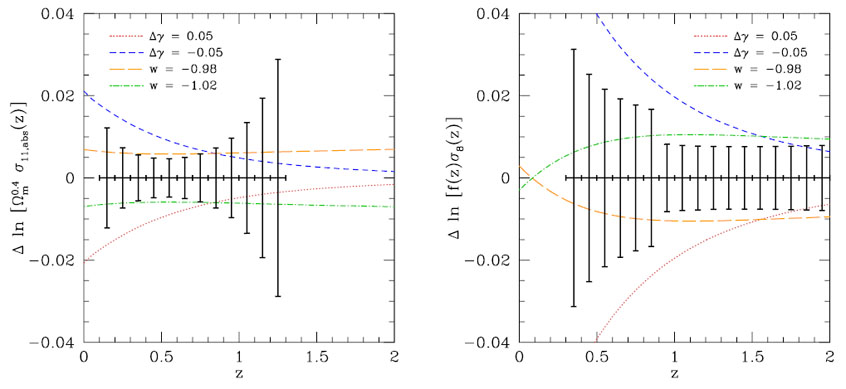 |
Figure 53. Forecast errors for fiducial Stage IV cluster (left) and RSD (right) programs, with the assumptions described in the text. Curves show the predicted deviations from our fiducial ΛCDM model for CMB-normalized models with 1 + w = ± 0.02 and Δγ = ± 0.05. |
The RSD error bars in Figure 53 are those shown previously by the lower solid curve in Figure 31, computed with the forecasting code of White et al. (2009). They assume a galaxy sample like that of our fiducial BAO program out to z = 2 and full use of information up to comoving k = kmax = 0.2 h Mpc-1 at each redshift. The sharp change in errors at z = 0.9 is due to the assumed drop in bias factor as surveys transition from absorption-line galaxies to emission-line galaxies. The aggregate precision on f(z) σ8(z) is 0.22%, again comparable to that of our other fiducial programs. The ranges z > 1.4 and z < 1.4 make equal contributions to this precision. As discussed in Section 7.2, we expect the dominant systematic uncertainty for RSD to lie in theoretical prediction of the RSD signal in the presence of non-linear gravitational evolution and galaxy bias, not the measurements themselves. To realize the full statistical power of Stage IV galaxy redshift surveys, these theoretical uncertainties must be controlled at the 0.2%-level. The White et al. (2009) forecasts, which assume that kmax scales with the non-linear wavelength knl(z) of the matter power spectrum, yield smaller errors at high redshift and an aggregate precision of 0.10%.
Curves in Figure 53 again show the effect of isolated parameter changes with 1 + w = ± 0.02 and Δγ = ± 0.05. In isolation, either of these changes would be strongly ruled out by either the fiducial cluster program or the fiducial RSD program with the assumptions adopted here. For clusters, the impact of the w changes is comparable to the 1σ error bar per Δz = 0.1 redshift bin over the range 0.2 < z < 0.8. The impact of Δγ changes exceeds the 1σ error at all z < 0.8. For RSD, the Δγ = ± 0.05 impact exceeds the 1σ per-bin error at all z < 1.7. In these CMB-normalized models, where changes to w and Ωm have counteracting effects on f(z), the sensitivity of RSD to a constant-w change is greatest at high redshifts. The impact of Δw = ± 0.02 exceeds the per-bin 1σ error for z ≥ 0.9.
Quantities like the DETF FoM and errors on Δγ or lnG9 are useful for optimizing choices in a well defined experimental program, e.g., area vs. depth or the value of different target classes in a spectroscopic survey. However, since we have little idea where deviations from GR+Λ are likely to show up (if they are there at all), we think that aggregate precision, including the effects of systematics, is a comparably useful tool for providing seat-of-the-pants guidance in a more general situation. For a given level of aggregate precision, a measurement at low redshift will typically have more direct sensitivity to dark energy, a measurement at high redshift will typically have more direct sensitivity to curvature, and measurements over a range of redshifts are needed to constrain dark energy evolution. However, given the degeneracies among parameters (especially w, Ωm, and Ωk) and the powerful impact of CMB constraints, it is difficult to identify a specific redshift range as the optimal one to probe. For a given method and a given facility, it makes sense to start where the pickings are easy, in terms of gaining precision relative to existing knowledge, and move to more difficult terrain when required. This assessment must also include consideration of where one can most readily control systematics, which is often but not always at low redshift. Extending the redshift range of a method increases leverage for breaking degeneracies and constraining dark energy evolution, but the more important impact is often to improve the method's aggregate precision by bringing in measurements with decorrelated errors. As we have emphasized repeatedly, a full program should employ multiple methods to take advantage of their complementary information content and redshift sensitivity and to cross-check for unrecognized systematics. Fortunately, Figures 52 and 53 show that several methods have the potential to achieve 0.1-0.3% aggregate precision in Stage IV experiments, a dramatic improvement on the ~ 1-5% precision that represents the current state of the art for these methods.
8.7. Prospects with Many Probes
Section 8.3 demonstrates the power of a combined CMB+SN+BAO+WL experimental program, while Sections 8.4 - 8.6 show that other probes could add substantial further sensitivity to dark energy or modified gravity. Drawing these results together, we show in Figure 54 the result of combining our fiducial CMB+SN+BAO+WL programs with representative performance estimates for clusters, redshift-space distortions, and direct H0 measurement. (While the AP test could also play an important role, we consider current understanding of its systematic uncertainty too limited to allow even representative performance estimates.) Top, middle, and bottom panels show inverse errors on wp, wa, and Δγ, respectively, assuming a w0-wa model with G9 and Δγ as beyond-GR growth parameters. Black bars show the results of combining all of these probes, while colored bars show the cumulative impact of successively omitting individual probes (see further explanation below).
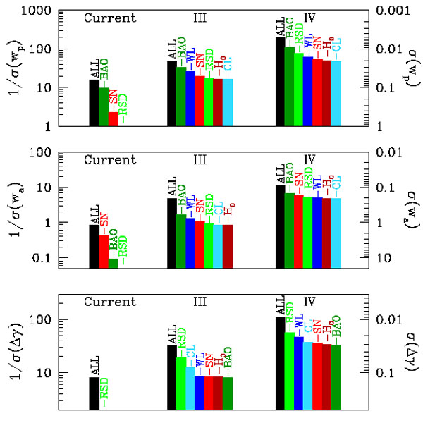 |
Figure 54. Forecasts for inverse 1σ errors (left axis; errors themselves on the right axis) on wp, wa, and Δγ from combining our fiducial CMB+SN+BAO+WL programs with additional constraints from redshift-space distortions (RSD), clusters (CL), and direct H0 measurements. See text for a description of the errors assumed for Current (left), Stage III (middle), and Stage IV (right) forecasts. Black bars show the results of combining all of these probes. Colored bars show the cumulative impact of dropping probes in succession ("-BAO" should be read as "minus BAO," for example). When a Stage IV probe is "dropped" it is set to its Stage III precision, and when a Stage III probe is "dropped" it is set to its current precision. CMB constraints are always retained. |
For Stage IV we assume our fiducial CMB, SN, BAO, and WL constraints, the cluster and RSD constraints described in Section 8.6 (Fig. 53), and an H0 constraint with precision of 1%. For Stage III we adopt the CMB+SN+BAO+WL errors summarized in Table 7. (Note, in particular, that our assumed Stage III SN errors are 0.02 mag per Δz = 0.2 bin and our Stage IV errors are 0.01 mag per bin, with the same error for the local calibrator sample at z = 0.05. For these plots, though not for others in the paper, we also include the Union2 SN constraints when computing Stage III and Stage IV.) For Stage III clusters we assume 5000 deg2 and a source density of 10 arcmin-2 for mass calibration (both appropriate to DES), while keeping the mass threshold at 2 × 10¹⁴ M⊙. For H0 we assume 2% errors, and for RSD we take the White et al. (2009) forecasts for BOSS. Finally, for current data we take WMAP CMB errors, Union2 SN errors, and the BAO data and errors described in Section 4.2. We adopt the RSD errors reported by Blake et al. (2011a) from WiggleZ (see Section 7.2). We also include a 3% error on H0, and a 4% error on σ8 Ωm0.4 to represent clusters and weak lensing (see Section 6.2).
Beginning with the black bars representing the full combinations, we see that these projections predict improvements of more than an order-of-magnitude for each of the three parameters — wp, wa, and Δγ — between current knowledge and Stage IV results. These combinations yield 1σ errors of approximately 0.005 on wp, 0.1 on wa, and 0.01 on Δγ, testing the ΛCDM model far more stringently than it has been tested to date. Stage III projections are roughly the geometric mean of current and Stage IV constraints in all cases.
It is interesting to ask what the different methods contribute to this performance, but there is no unique way to decompose a constraint into a sum of individual contributions, and the apparent relative importance of different components depends on how the decomposition is done. We have attempted one form of "even-handed" decomposition by dropping individual probes in succession, beginning with the probe whose omission causes the largest increase in the parameter error, then the probe that causes the largest increase after the first probe has already been dropped, and so forth. However, when we "drop" a probe we do not omit it entirely; rather, we set the error for that probe in the Stage IV forecast equal to the value we previously assumed for the Stage III forecast, or we set the error in the Stage III forecast equal to the value adopted for current data. Thus, for example, the dark green bar in the upper right shows the impact on σ(wp) of replacing the Stage IV BAO constraints with the Stage III BAO constraints. The light green bar next to it shows the impact of also setting the RSD constraint to the Stage III value, the dark blue bar the impact of also setting the WL constraint to the Stage III value, and so forth. To give one more example, the light blue bar in the middle of the bottom panel shows the error on Δγ using Stage III WL+SN+BAO+H0 but current constraints for RSD and clusters. If the Stage III WL improvement is also dropped (dark blue bar) then there is no improvement over current knowledge of Δγ because none of the remaining probes (SN, BAO, H0) directly measures structure growth. We always include CMB constraints, with WMAP9 errors for current and Planck errors for Stage III and Stage IV. By construction, the rightmost colored bar for a given stage matches the black bar of the previous stage, since we have then set all probes back to their value in the previous stage.
We caution against reading too much into the ordering of probes in Figure 54 because it depends in detail on our assumptions about the expected errors of the individual components; furthermore, a probe only gains in this plot based on its differential improvement between current performance and Stage III or between Stage III and Stage IV. The detailed examination of CMB+SN+BAO+WL in Tables 8 - 10 and the associated figures provides much more nuanced information. These caveats notwithstanding, Figure 54 demonstrates several interesting points. In present data, BAO make the largest contribution to wp constraints and SNe to wa constraints, 83 though it is really the combination of the two with CMB data that is required to achieve interesting constraints in a model space that allows wp, wa, and Ωk to vary simultaneously. BAO become more powerful in our fiducial Stage III and Stage IV programs, making the largest contribution to both the wp and wa constraints. Current constraints on Δγ rely entirely on RSD, as the cluster constraint on σ8 Ωm0.4 is degenerate with G9. With our adopted error forecast, RSD remains the most powerful contributor to Δγ constraints at Stage III and Stage IV, outweighing both WL and clusters. Indeed, with these errors Stage IV RSD also makes an important contribution to the wp measurement. WL and clusters make significant contributions to Δγ constraints but have limited impact on wp and wa.
Figure 55 shows two variants on the fiducial Stage IV case. In the middle column we consider a combined program with SN errors improved by a factor of two and the optimistic WL systematics. The forecast errors on wp, wa, and Δγ shrink by 6%, 21%, and 8%, respectively. WL and SN now leapfrog RSD as contributors to the wp error, though they still contribute less than BAO. The improvement in wa is driven by the supernova improvement, though BAO remains the largest contributor. The right column shows the effect of, additionally, doubling the errors on BAO and RSD, since our fiducial assumptions for these programs are perhaps overoptimistic compared to the capabilities of planned Stage IV experiments. The forecast errors are larger than they are for the fiducial case but by moderate amounts, 20% (wp), 14% (wa), and 28% (Δγ). WL leapfrogs BAO to become the strongest contributor to wp precision, while SN and WL both leapfrog BAO for wa. With doubled measurement errors, RSD makes only a modest contribution to the parameter constraints, even for Δγ.
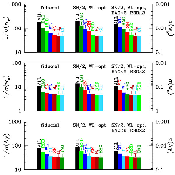 |
Figure 55. Like Figure 54, but showing variations on the Stage IV fiducial program. The middle column shows forecasts with the optimistic WL systematics and SN errors reduced by a factor of two. The right column shows the effect of, additionally, doubling the errors on RSD and BAO. The left column repeats the fiducial case from Fig. 54 for reference. |
Perhaps the most important message to take from Figures 54 and 55 is that these six probes together with CMB measurements provide a tight web of constraints on cosmic acceleration models, and that even if one or two methods prove disappointing, there are others (including ones not shown in this plot) to take up slack. We have focused much of our review on the stiff challenges of controlling systematic errors at the level demanded by future dark energy experiments. However, given the ingenuity of the community in devising and refining analysis methods, we are optimistic that the powerful data sets provided by these experiments will ultimately lead to constraints at the high end of our forecasts.
74 This is equivalent to assuming linear theory sample variance over a fractional volume 25%/1.82 = 7.7%. Back.
75 Since we neglect magnification bias, some of these spectra, e.g. the correlation of high-redshift galaxies with low-redshift shear, are zero for all cosmological models. Back.
76 i.e. with sufficiently wide prior that no significant information remains. Back.
77 Note that our wi parameterization has exactly (0.25 - 0.1) / 0.025 = 6 bins at 3 < z < 9 and 30 bins at z < 3. PC 31 parameterizes variations in the lowest redshift bin w1, which is poorly constrained as discussed in Section 8.3.3. Back.
78 This partly depends on the choice of fiducial model at which the Fisher matrix used to construct the PCs is computed. Taking a fiducial model with a larger dark energy density at high redshift than in ΛCDM makes the low-redshift PC shapes more sensitive to assumptions about the high-redshift equation of state (e.g., de Putter and Linder 2008). Back.
79 Note, however, that either decreased SN errors or increased BAO errors for any of these forecasts would reduce the difference between the predictions at z < 1 and at z > 1. Back.
80 Specifically, that forecast assumes uncorrelated systematic errors of 0.01(1 + z) / 1.8 mag in 16 Δz = 0.1 redshift bins out to z = 1.7. The total errors have roughly comparable statistical and systematic contributions. Back.
81 Schlegel et al. (2011) use a different convention, quoting nP for the redshift-space power spectrum at k = 0.14 h Mpc-1 and μ = 0.6 instead of the real-space power spectrum at k = 0.2 h Mpc-1. We have quoted the numbers from their Table 2.3 as is, with no conversion to our nP convention and no independent assessment of the sampling density the instrument is likely to achieve. Back.
82 These models have h = 0.7030 (w = -0.98), h = 0.7171 (w = -1.02), h = 0.7157 (Ωk = 0.001) and h = 0.7045 (Ωk = -0.001). Other parameters can be computed from the conditions Ωb h2 = 0.02268, Ωc h2 = 0.1119, and Ωϕ = 1 - Ωc - Ωb - Ωk. Back.
83 Interestingly, the roles of BAO and SNe in the current wp constraint are reversed relative to the original arXiv posting of our article because of the inclusion of the new SDSS DR7 and BOSS measurements, both published in 2012. Back.