6. LIMITS ON N_eff

Before concluding, we consider a one-parameter extension of SBBN by allowing the number of relativistic degrees of freedom to differ from the Standard Model value of N_ν = 3 and N_eff = 3.046. Opening this degree of freedom has an impact on both the CMB and BBN. In Fig. 6, the thinner contours show the 2D likelihood distribution in the (η, N_ν) plane, using Planck data marginalizing over the CMB Y_p. We see that the CMB N_ν values are nearly uncorrelated with η. The thicker contours include BBN information and are discussed below.

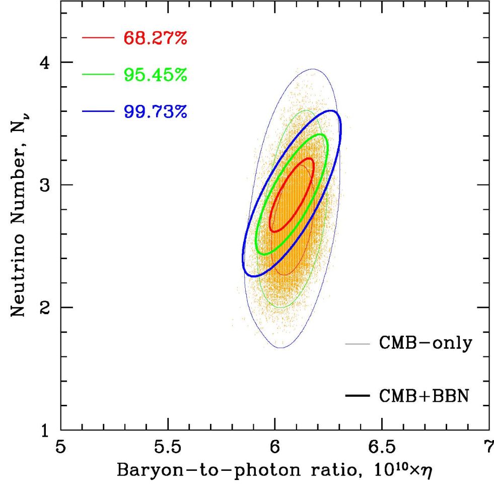Figure 6. The 2D likelihood function contours derived from the Planck Markov Chain Monte Carlo base_nnu_yhe [113], marginalized over the CMB Yp (points). Thin contours are for CMB data only, while thick contours use the BBN Yp(η) relation, assuming no observational constraints on the light elements. We see that that whereas in the CMB-only case Nν and η are almost uncorrelated, in the CMB+BBN case a stronger correlation emerges.

Turning to the effects of N_ν on BBN, eqs. (1) – (3) show that increasing the number of neutrino flavors leads to an increased Hubble parameter which in turn leads to an increased freeze-out temperature, T_f. Since the neutron-to-proton ratio at freeze-out scales as (n / p) ≃ e^{−Δ m / T_f}, higher T_f leads to higher (n / p) and thus higher Y_p [122]. As a consequence, one can establish an upper bound to the number of neutrinos [123] if in addition one has a lower bound on the baryon-to-photon ratio [25] as the helium abundance also scales monotonically with η. The dependence of the helium mass fraction Y on both η and N_ν can be seen in Figure 7 where we see the calculated value of Y for N_ν= 2, 3 and 4 as depicted by the blue, green and red curves respectively. In the Figure, one clearly sees not only the monotonic growth of Y with η, but also the strong sensitivity of Y with N_ν. The importance of a lower bound on η (or better yet fixing η) is clearly apparent in setting an upper bound on N_ν. Prior to CMB determinations of η, the lower bound on η could be set using a combination of D and ³He observations enabling a limit of N_ν< 4 [124] given the estimated uncertainties in Y_p at the time. More aggressive estimates of an upper bound on the helium mass fraction led to tighter bounds on N_ν [1, 125, 109]. The bounds on N_ν became more rigorous when likelihood techniques were introduced [109, 126, 127, 128, 5, 57, 129].

While the dependence of Y_p on N_ν is well documented, we also see from Fig. 7, there is a non-negligible effect on D and ⁷Li from changes in N_ν [5]. In particular, while the sensitivity of D to N_ν is not as great as that of Y_p, the deuterium abundance is measured much more accurately and as a result the constraint on N_ν is now due to both abundance determinations as can be discerned from Table 5.

Figure 7. The sensitivity of the light element predictions to the number of neutrino species, similar to Figure 1. Here, abundances shown by blue, green, and red bands correspond to calculated abundances assuming Nν = 2, 3 and 4 respectively.

By marginalizing over the baryon density, we can form 1-d likelihood functions for N_ν. These are shown in Figure 8. In the left panel, we show the CMB-only result by the blue curve. Recall that this uses no BBN correlation between the baryon density and helium abundance. While the peak of the likelihood for this case is lowest of the cases considered (N_ν = 2.67) its uncertainty (≈ 0.30) makes it consistent with the Standard Model. The position of the peak of the likelihood function is given in Table 5 for this case as well as the other cases considered in the Figures. In contrast the red curve shows the limit we obtain purely from matching the BBN calculations with the observed abundances of helium and deuterium. In this case, the fact that the peak of the likelihood function is at N_ν = 2.85 can be traced directly to the fact that the central helium abundance is Y_p = 0.2449. Given the sensitivity of Y_p to N_ν found in Eq. 13, the drop in N_ν from the Standard Model value of 3.0, compensates for a helium abundance below the Standard Model prediction closer to 0.247. Nevertheless, the uncertainty again places the Standard Model within 1 σ of the distribution peak. The remaining cases displayed (in green) correspond to combining the CMB data with BBN. There are 4 green curves in the left panel and these have been isolated in the right panel for better clarity. As one can see, once one combines the BBN relation between helium and the baryon density, the actual abundance determinations have only a secondary effect in determining N_ν which takes values between 2.88 and 2.91. Using the CMB, BBN and the abundances of both D and ⁴He, yields the tightest constraint on the number of neutrino flavors N_ν = 2.88 ± 0.16, again consistent with the Standard Model ⁵. It is interesting to note, that because of the drop in Y_p in the most recent analysis [39], the 95% CL upper limit on N_ν is 3.20.

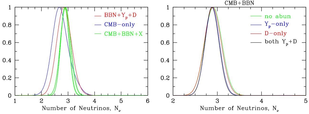Figure 8. The marginalized distributions for the number of neutrinos, given different combinations of observational constraints. The left panel shows the likelihood function the case where only CMB data is used (blue), only BBN and abundance data is used (red) and when a combination of BBN and CMB data is used (green). The four green curves are shown again in the right panel for better clarity.

It is also possible to marginalize over the number of neutrino flavors and produce a 1-d likelihood function for η₁₀ as shown in Figure 9. In the left panel, the broad distribution shown in red corresponds to the BBN plus abundance data constraint using no information from the CMB. Here the baryon density is primarily determined by the D/H abundance. When the CMB is added, the uncertainty in η drops dramatically (from 0.23 to 0.06 or 0.07) independent of whether abundance data is used. The 5 green curves are almost indistinguishable and are shown in more detail in the right panel. Once again the peak of the likelihood distributions are given in Table 5. The values of η are slightly lower than the Standard Model results discussed above. This is due to the additional freedom in the likelihood distribution afforded by the additional parameter,

Figure 9. The marginalized distributions for the baryon to photon ratio (η), given different combinations of observational constraints.

For completeness, we also show 2-d likelihood contours in the η₁₀ − N_ν plane in Fig. 10. The three panels show the effect of the constraints imposed by the helium and deuterium abundances. In the first panel, only the helium abundance constraints are applied. The thinner open curves are based on BBN alone. They appear open as the helium abundance alone is a poor baryometer as has been noted several times already. Without the CMB, the helium abundance data can produce an upper limit on N_ν of about 4 and depends weakly on the value of η. When the CMB data is applied, we obtain the thicker closed contours. The precision determination of η from the anisotropy spectrum correspondingly produces a very tight limit in N_ν. Here, we see clearly that the Standard Model value of N_ν = 3 falls well within the 68% CL contour.

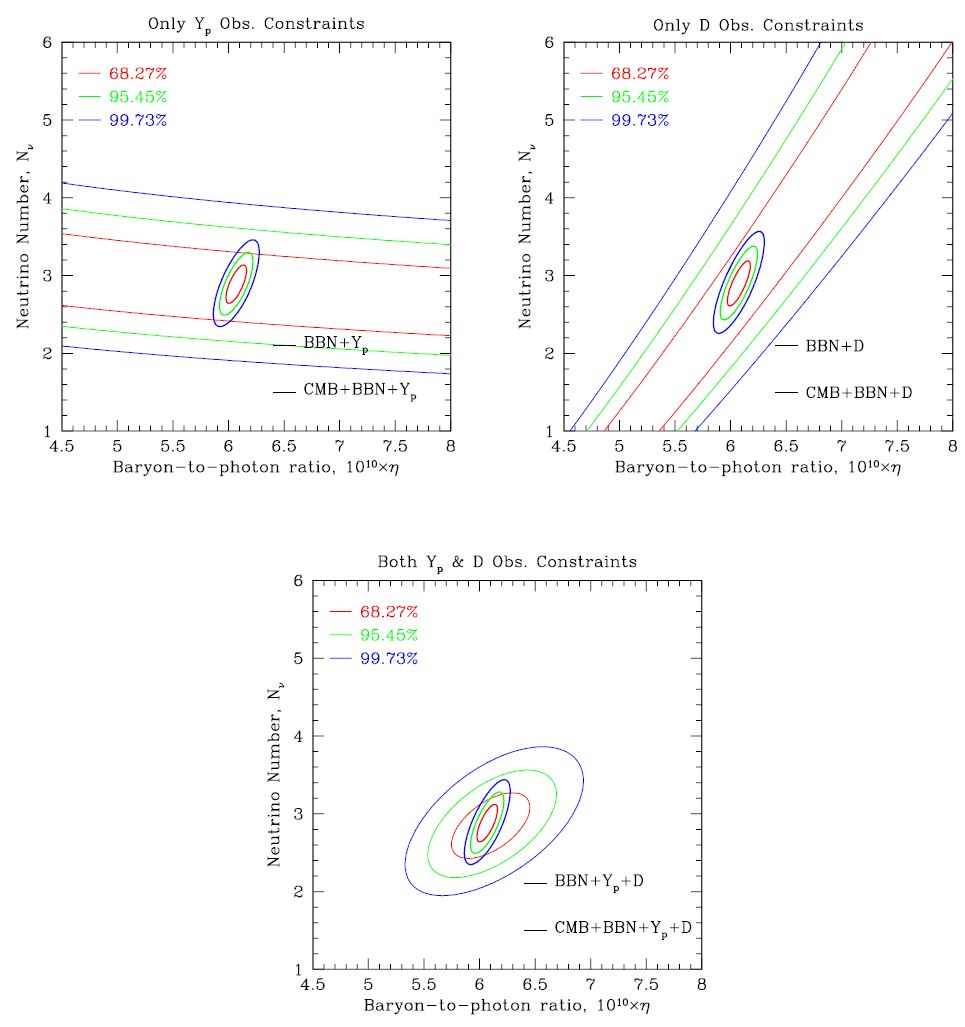Figure 10. The resulting 2-dimensional likelihood functions for the baryon to photon ratio (η) and the number of neutrinos (Nν), marginalized over the helium mass faction Yp, assuming different combinations of observational constraints on the light elements.

The next panel of Figure 10 shows the likelihood contours using the deuterium abundance data. Once again, the thin open curves are based on BBN alone. In this case, they appear open as the deuterium abundance is less sensitive to N_ν, though we do note that the contours are not vertical and do show some dependence on N_ν as discussed above. In contrast to ⁴He, for fixed N_ν, the deuterium abundance is capable of fixing η relatively precisely. Of course when the CMB data is added, the open contours collapse once again into a series of narrow ellipses.

The last panel of Figure 10 shows the likelihood contours using both the ⁴He and D/H data. In this case, even without any CMB input, we are able to obtain reasonably strong constraints on both η and N_ν as seen by the thin and larger ellipses. When the CMB data is added we recover the tight constraints which are qualitatively similar to those in the previous two panels.

Finally, above in Figure 6, we show the 2-dimensional likelihood function using either CMB only (the thin outer curves which trace the density of models results of the Monte-Carlo), or the combination of CMB and BBN (tighter and thicker curves). In the latter case, no abundance data is used.

⁵ Of all the cases considered, the one that can best be compared with the results presented by the Planck collaboration [6] is the case CMB+BBN+D. We find N_eff = 2.94 ± 0.38 (2 σ) while they quote N_eff = 2.91 ± 0.37. While we obtain similar results to other cases, direct comparison is complicated not only by the slight difference in the η−Y relation due to different BBN codes, but also by the adopted value for primordial ⁴He. Back.