4.1. Monte-Carlo Predictions for the Light
Elements
The dominant source of uncertainty in the BBN light-element
predictions stem from experimental uncertainties of nuclear reaction
rates. We propagate these uncertainties by randomly drawing rates
according their adopted probability distributions for each BBN
evaluation. We choose a Monte Carlo of size N = 10000, keeping
the error in the mean and error in the error
at the 1% level. It is important that we use the same random numbers for
each set of parameters (η, Nν). This helps
remove any extra noise from the Monte Carlo predictions and allows for
smooth interpolations between parameter points.
For each grid point of parameter values we calculate the means and
covariances of the light element abundance predictions. We add the
1/√N errors in
quadrature to our evaluated uncertainties on the light element
predictions. We have examined the light element abundance distributions,
by calculating higher
order statistics (skewness and kurtosis), and by histogramming the resultant
Monte Carlo points and verified that they are well-approximated with
log-normal or gaussian distributions.
In standard BBN, the baryon-to-photon ratio (η) is the only free
parameter of the theory. Our Monte Carlo error propagation is
summarized in Figure 1, which plots the light
element abundances as a function of the baryon density (upper scale) and
η (lower scale). The abundance for He is shown as the mass
fraction Y, while the abundances of
the remaining isotopes of D, 3He, and 7Li are
shown as abundances by number relative to H.
The thickness of the curves show the ± 1 σ spread in the
predicted abundances. These
results assume Nν= 3 and the current measurement
of the neutron lifetime τn = 880.3 ± 1.1 s.
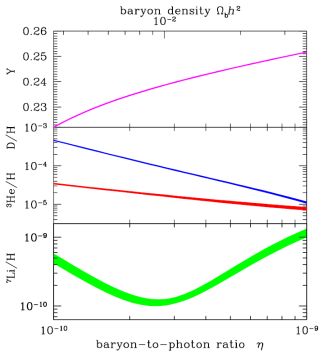 |
Figure 1. Primordial abundances of the
light nuclides as a function of cosmic baryon content, as predicted by
SBBN (“Schramm plot”). These
results assume Nν = 3 and the current
measurement of the neutron lifetime τn = 880.3 ±
1.1 s. Curve widths show 1−σ errors. |
Using a Monte Carlo approach also allows us to extract sensitivities
of the light element predictions to reaction rates and other
parameters. The sensitivities are defined as the logarithmic
derivatives of the light element abundances with respect to each
variation about our fiducial model parameters
[112],
yielding a simple relation for extrapolating about the fiducial model:
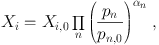 |
(12) |
where Xi represents either the helium mass fraction or
the abundances of the other light elements by number. The
pn represent input quantities to the BBN calculations
(η, Nν, τn) and the
gravitational constant Gn as well key nuclear rates
which affect the abundance Xi. pn,0
refers to our standard input value. The information contained
in Eqs. (13-17) are neatly summarized in Table 3.
 |
(13) |
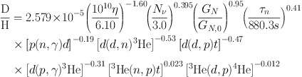 |
(14) |
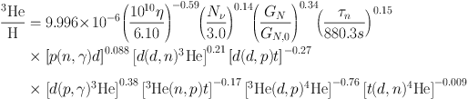 |
(15) |
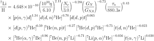 |
(16) |
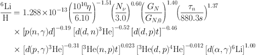 |
(17) |
Table 3. This table contains the
sensitivities, αn's defined in Eq. 12 for each of the
light element abundance predictions, varied with respect to key
parameters and reaction rates.
| Variant |
Yp |
D/H |
3He/H |
7Li/H |
6Li/H |
| η (6.1 × 10⁻¹⁰) |
0.039 |
-1.598 |
-0.585 |
2.113 |
-1.512 |
| Nν (3.0) |
0.163 |
0.395 |
0.140 |
-0.284 |
0.603 |
| Gn |
0.354 |
0.948 |
0.335 |
-0.727 |
1.400 |
| n-decay |
0.729 |
0.409 |
0.145 |
0.429 |
1.372 |
| p(n,γ)d |
0.005 |
-0.194 |
0.088 |
1.339 |
-0.189 |
| 3He(n,p)t |
0.000 |
0.023 |
-0.170 |
-0.267 |
0.023 |
| 7Be(n,p)7Li |
0.000 |
0.000 |
0.000 |
-0.705 |
0.000 |
| d(p,γ)3He |
0.000 |
-0.312 |
0.375 |
0.589 |
-0.311 |
| d(d,γ)4He |
0.000 |
0.000 |
0.000 |
0.000 |
0.000 |
| 7Li(p,α)4He |
0.000 |
0.000 |
0.000 |
-0.056 |
0.000 |
| d(α,γ)6Li |
0.000 |
0.000 |
0.000 |
0.000 |
1.000 |
| t(α,γ)7Li |
0.000 |
0.000 |
0.000 |
0.030 |
0.000 |
| 3He(α,γ)7Be |
0.000 |
0.000 |
0.000 |
0.963 |
0.000 |
| d(d,n)3He |
0.006 |
-0.529 |
0.213 |
0.698 |
-0.522 |
| d(d,p)t |
0.005 |
-0.470 |
-0.265 |
0.065 |
-0.462 |
| t(d,n)4He |
0.000 |
0.000 |
-0.009 |
-0.023 |
0.000 |
| 3He(d,p)4He |
0.000 |
-0.012 |
-0.762 |
-0.752 |
-0.012 |
4.2. The Neutron Mean Life
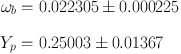
As noted in the introduction, the value of the neutron mean life has
had a turbulent history. Unfortunately, the predictions of SBBN
remain sensitive to this quantity. This sensitivity is displayed in the
scatter plot of our Monte Carlo error propagation with fixed
η = 6.10 × 10⁻¹⁰
in Figure 2. The correlation between the neutron
mean lifetime and 4He abundance prediction is clear. The
correlation is
not infinitesimally narrow because other reaction rate uncertainties
significantly contribute to the total uncertainty in 4He.
 |
Figure 2. The sensitivity of the
4He abundance to the neutron mean life, as shown through a
scatter plot of our Monte Carlo error propagation. |
4.3. Planck Likelihood Functions
For this paper, we will need to consider two sets of Planck
Markov Chain data, one for standard BBN (SBBN) and one for non-standard
BBN (NBBN). Using the Planck Markov chain data
[113],
we have constructed the
multi-dimensional likelihoods for the following extended parameter
chains, base_yhe and base_nnu_yhe, for the
plikHM_TTTEEE_lowTEB dataset.
As noted earlier, we do not use the Planck base chain, as it
assumes a BBN relationship
between the helium abundance and the baryon density.
From these 2 parameter sets we have the following 2- and 3-dimensional
likelihoods from the CMB:
 PLA−base_yhe(ωb,
Yp)
and PLA−base_nnu_yhe(ωb,
Yp, Nν).
The 2-dimensional base_yhe likelihood is well-represented by
a 2D correlated gaussian distribution, with means and standard
deviations for the baryon density and 4He mass fraction
PLA−base_yhe(ωb,
Yp)
and PLA−base_nnu_yhe(ωb,
Yp, Nν).
The 2-dimensional base_yhe likelihood is well-represented by
a 2D correlated gaussian distribution, with means and standard
deviations for the baryon density and 4He mass fraction
 |
(18) (19) |
and a correlation coefficient
r ≡
cov(ωb, Yp) /
√var(ωb)
var(Yp) = +0.7200.
The two parameter data can be marginalized to yield 1-dimensional
likelihood functions for η. The peak and 1-σ spread in
η is given in the first row of Table 4.
The following rows correspond to different determinations of η. In
the second-fourth rows, no CMB data is used. That is, we fix η
only from the observed abundances of 4He, D or both.
Notice for example, in row 2, the value for η is low and has a
huge uncertainty. This is due to the slightly low value for the
observational abundance (7) and the logarithmic dependence of
Yp on η. We see again that BBN +
Yp is a poor baryometer. This will be described in
more detail in the following subsection. Row 5, uses the BBN relation
between η and Yp, but no observational input
from Yp is used. This is closest to the
Planck determination found in
[6],
though here Yp was taken to be free
and the value of η in the Table is a result of marginalization
over Yp.
This accounts for the very small difference in the results for η:
η10 = 6.09 (Planck);
η10 = 6.10 (Table 4). Rows 6-8
add the observational determinations of
4He, D and the combination. As one can see, the inclusion of
the observational data does very little to affect the determination of
η and thus we use η10 = 6.10
as our fiducial baryon-to-photon ratio.
Table 4. Constraints on the baryon-to-photon
ratio, using different combinations of observational constraints. We
have marginalized over Yp to create 1D η
likelihood distributions.
| Constraints Used |
η × 1010 |
| CMB-only |
6.108 ± 0.060 |
| BBN+Yp |
4.87−1.54+2.46 |
| BBN+D |
6.180 ± 0.195 |
| BBN+Yp+D |
6.172 ± 0.195 |
| CMB+BBN |
6.098 ± 0.042 |
| CMB+BBN+Yp |
6.098 ± 0.042 |
| CMB+BBN+D |
6.102 ± 0.041 |
| CMB+BBN+Yp+D |
6.101 ± 0.041 |
The 3-dimensional base_nnu_yhe likelihood is not
well-represented by a simple 3D correlated gaussian distribution, but
since these distributions are single-peaked we can correct for the
non-gaussianity via a 3D Hermite expansion about a 3D correlated
gaussian base distribution. Details of this prescription will be given
in the Appendix.
The calculated mean values and standard
deviations for these distributions are:
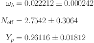 |
(20) (21) (22) |
These values correspond to the peak of the likelihood distribution using
CMB data alone. That is, no use is made of the correlation between the
baryon density and the helium abundance through BBN.
For this reason, the helium mass fraction is found to be rather
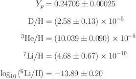
high. Our value of Yp = 0.261 ± 0.36 (2σ)
can be compared with the value given by the Planck
collaboration
[6] of
Yp = 0.263−0.37+0.34.
In this case, we marginalize to form a 2-d likelihood function to
determine both η and Neff.
As in the 1-d case discussed above, we can determine η and
Nν using CMB data
alone. This result is shown in row 1 of Table 5
and does not use any correlation between η and
Yp. Note that the value of Nν
given here differs from that in Eq. (21) since the value in the Table
comes from a marginalized likelihood function, where as the value in the
equation does not. Row 2, uses only BBN and the observed abundances
of 4He and D with no direct information from the CMB. Rows
3-6 use the combination of the CMB data, together with the BBN relation
between η and Yp with and without the
observational abundances as denoted. As one can see, opening up the
parameter space to allow Nν to float
induces a relatively small drop η (by a fraction of 1 σ) and
the peak for Nν is below
the Standard Model value of 3 though consistent with that value within 1
σ.
Table 5. The marginalized most-likely values
and central 68.3% confidence limits on the baryon-to-photon ratio and
effective number of neutrinos, using different combinations of
observational constraints.
| Constraints Used |
η10 |
Nν |
| CMB-only |
6.08±0.07 |
2.67−0.27+0.30 |
| BBN+Yp+D |
6.10±0.23 |
2.85±0.28 |
| CMB+BBN |
6.08±0.07 |
2.91±0.20 |
| CMB+BBN+Yp |
6.07± 0.06 |
2.89± 0.16 |
| CMB+BBN+D |
6.07±0.07 |
2.90±0.19 |
| CMB+BBN+Yp+D |
6.07± 0.06 |
2.88±0.16 |
We note that we have been careful to use the appropriate relation
between η and ωb via Eq. 11. Also, in our NBBN
calculations we formally use the number of neutrinos, not the
effective number of neutrinos, thus demanding the relation:
Neff = 1.015333Nν. For the 2D
base_yhe CMB likelihoods,
we include the higher order skewness and kurtosis terms to
more accurately reproduce the tails of the distributions.
4.4. Results: The Likelihood Functions
Applying the formalism described above, we derive the likelihood functions
for SBBN and NBBN that are our central results.
Turning first to SBBN, we fix Nν = 3
and use the Planck determination of η as
the sole input to BBN in order to derive CMB+BBN
predictions for each light element.
That is, for each light element species Xi we
evaluate the likelihood
 |
(23) |
where
bbn(η;
{Xi}) comes from our BBN
Monte Carlo, and where we use the η − ωb
relation in eq. (11).
In the case of 4He, we use only the CMB η to determine
the Xi = Yp,BBN prediction and
compare this to the CMB-only prediction.
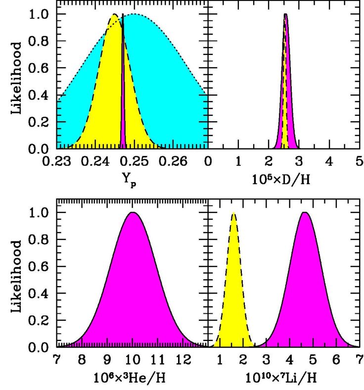
The resulting CMB+BBN abundance likelihoods appear
as the dark-shaded (purple, solid line) curves in
Figure 3,
which also shows the observational abundance constraints
(Section 3) in the light-shaded (yellow,
dashed-line) curves.
In panel (a), we see that the 4He BBN+CMB likelihood is
markedly more narrow than its observational counterpart,
but the two are in near-perfect agreement.
The medium-shaded (cyan, dotted line) curve in this panel
is the CMB-only Yp prediction,
which is the least precise but also completely consistent
with the other distributions. Panel (b) displays the dramatic
consistency between
the CMB+BBN deuterium prediction and the observed high-z abundance.
Moreover, we see that the D/H observations
are substantially more precise than the theory.
Panel (c) shows the primordial 3He prediction, for which
there is no reliable observational test at present.
Finally, panel (d) reveals a sharp discord between
the BBN+CMB prediction for 7Li and the observed primordial
abundance–the two likelihoods are essentially disjoint.
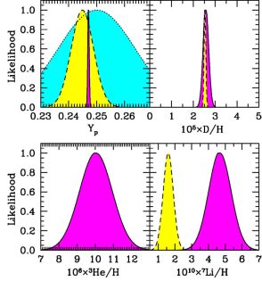 |
Figure 3. Light element predictions using
the CMB determination of the cosmic baryon density. Shown are
likelihoods for each of the light nuclides, normalized to show a
maximum value of 1. The solid-lined, dark-shaded (purple) curves are
the BBN+CMB predictions, based on Planck inputs as discussed
in the text. The dashed-lined, light-shaded
(yellow) curves show astronomical measurements
of the primordial abundances, for all but 3He where
reliable primordial abundance measures do not exist. For
4He, the dotted-lined, medium-shaded (cyan) curve shows
the CMB determination of 4He. |
Figure 3 represents not only a quantitative
assessment of the concordance of BBN, but also a test of the
standard big bang cosmology.
If we limit our attention to each element in turn,
we are struck by the spectacular agreement between
D/H observations at z ∼ 3 and the BBN+CMB predictions
combining physics at z ∼ 1010 and z
∼ 1000. The consistency among all three Yp
determinations is similarly remarkable, and the joint concordance
between D and 4He represents a non-trivial success of the
hot big bang model. Yet this concordance is not complete:
the pronounced discrepancy in 7Li measures
represents the “lithium problem” discussed below
(Section 5). This casts a shadow of doubt
over SBBN itself, pending a firm resolution of the lithium problem,
and until then the BBN/CMB concordance remains an
incomplete success for cosmology.
Quantitatively, the likelihoods in Fig. 3
are summarized by the predicted abundances
 |
(24) (25) (26)
(27) (28) |
where the central value give the mean, and the error the 1σ variance.
The slightly differences from the values in
Table 2 arise due to the Monte Carlo
averaging procedure here as opposed to evaluating the abundance using
central values of all inputs at a single η.
We see that the BBN/CMB comparison is enriched now that
the CMB has achieved an interesting sensitivity to Yp
as well as η. This interplay is further illustrated in
Figure 4, which shows 2-D likelihood contours
in the (η, Yp) plane, still for fixed
Nν = 3.
The Planck contours show a positive correlation between
the CMB-determined baryon density and helium abundance.
Also plotted is the BBN relation for Yp(η), which
for SBBN is a zero-parameter curve that is very tight even
including its small width due to nuclear reaction rate
uncertainties. We see that the curve
goes through the heart of the CMB predictions,
which represents a novel and non-trivial test of SBBN
based entirely on CMB data without any astrophysical input.
This agreement stands as a triumph for SBBN and the hot big bang,
and illustrates the still-growing power of the CMB
as a cosmological probe.
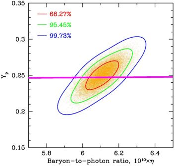 |
Figure 4. The 2D likelihood function
contours derived from the Planck
Markov Chain Monte Carlo base_yhe
[113]
with fixed Nν = 3 (points).
The correlation between Yp and η is evident.
The 3-σ BBN prediction for the helium mass fraction is shown with
the colored band. We see that including the BBN
Yp(η) relation significantly reduces
the uncertainty in η due to the CMB
Yp − η correlation. |
Thus far we have used the CMB η as an input to BBN;
we conclude this section by studying the constraints on η
when jointly using BBN theory, light-element abundances, and the CMB
in various combinations.
Figure 5 shows the η likelihoods
that result from a set of such combinations.
Setting aside at first the CMB,
the BBN+X curves show the combination of BBN theory
and astrophysical abundance observations,
BBN+X(η) =
∫bbn(η, X)
obs(X)
dX, with X ∈ (Yp, D /
H). The CMB-only curve marginalizes over the Planck
Yp values
CMB−only(η) =
∫PLA−base_yhe(ωb,
Yp) dYp
where we use the η−ωb relation
in eq. (11).
The BBN+CMB curve adds the BBN Yp(η) relation.
Finally, BBN+CMB+D also includes the observed primordial deuterium.
We see in Fig. 5 that of the primordial
abundance observations, deuterium is the only useful
“baryometer,” due to its
strong dependence on η in the Schramm plot
(Fig. 1
).
By contrast,