2. USING TIDAL DEBRIS TO PROBE THE GLOBAL POTENTIAL

As indicated in the introduction, adopting the simplifying (but ultimately incorrect) assumption that debris exactly traces a single orbit allows us to develop some intuition for how this data might be used. We can expand this intuition a little more by considering properties of orbits in different potentials. For example:

1. Orbits in a spherical potential are purely planar, while in oblate potentials, the orbital plane itself precesses with time. Figure 1 illustrates this by showing the orbital path (in red) and orbital pole (i.e., direction of angular momentum, in blue) in 3-D (top panels) and projected onto the plane of the sky (as viewed from the center of the parent galaxy — bottom panels) for the same orbit in spherical (left panels) and oblate (right panels) potentials. In the spherical case, the orbit aligns with a single plane on the sky and the pole appears as a single point. In the oblate case, the precession of the orbital plane is apparent as the orbital path not aligning with a single great circle and the direction of the pole evolving in time.

Figure 1. The left and right panels show (in red) external and internal views of orbital paths in spherical and oblate potentials respectively. External views are as seen from outside the galaxy; the center of the galaxy is shown by a small blue dot. Internal views are Aitoff projection all-sky maps, as seen from the galaxy center. The direction of the orbital pole is shown by the blue line in external views and blue dots (in the oblate case a moving dot) in the internal views. The position of the pole changes over time for the oblate case due to the precession of the orbital plane, but the position of the pole does not change for the spherical case.

2. Within the orbital plane, the precession of the angular position of apocenters reflects the radial density profile of the parent potential. Figure 2 (from Belokurov et al. 2014) shows this precession angle calculated for a variety of potentials and orbital eccentricities, with zero precession corresponding to the point-mass, Keplerian potential in which orbits are ellipses and the apocenters are coincident.

Figure 2. Potential profile dependence of the precession of turning points. The plot shows the angle between successive apocenters for potentials varying from logarithmic to Keplerian. The colors are for orbits of different eccentricity. Reproduced from Belokurov et al. (2014).

3. The eccentricity (or ratio of apocenter to pericenter) of the orbit for a given pericentric velocity is set by the overall depth of the potential.

We are now in a position to measure the attributes listed above for observed streams. For example, using debris from the (ongoing) destruction of the Sagittarius (Sgr) dwarf spheroidal (see Chapter 2 of this volume), we know the precession of the orbital plane (Majewski et al. 2003), the trends of velocity along the stream (Majewski et al. 2004), as well as the angular separation between successive apocenters (Belokurov et al. 2014). It is this level of detailed data that has enabled the first attempt to reconstruct the 3-dimensional shape and orientation of our Galactic dark matter halo (Law & Majewski 2010), or indeed of any galaxy in the Universe. However, significant controversy remains over what this reconstruction means, and this is inspiring a thorough and rigorous examination of how debris can robustly be used to measure potentials.

A multitude of approaches to exploiting our rich debris data sets to measure potentials have been proposed. They can be very broadly divided into two categories:

Predictive models predict the exact six-dimensional phase-space position and density of tidal debris from the progenitor's properties, orbit and parent galaxy potential. It is trivial to project the predictions of these models from phase-space to observables and hence to perform the comparison of data and model in coordinates where error distributions are well-understood. Hence these methods are the easiest for which to account for the effect of errors (or even missing dimensions of information) on any parameter estimates. However, they are also the most sensitive to biases that may result from incorrect assumptions in the model — in particular in how stars are distributed in the satellite. For example, a rotating satellite can produce tidal streams with centroids systematically offset from those produced by a non-rotating satellite (Peñarrubia et al. 2010).

Fundamental methods exploit some more general intrinsic property that debris obeys rather than matching the full density distribution in phase-space. Typically, these methods require few (if any) assumptions about the satellite's internal structure and may be less prone to such biases than predictive models. On the other hand, they always involve a non-trivial transformation from observed co-ordinates to perform a comparison with model predictions, so correcting for systematic and random biases on parameter estimates due to errors in observables is difficult, if not impossible.

Methods in both categories are reviewed in more detail below.

2.1. Predictive models

The most obvious example of a predictive model is an N-body simulation in which a ball of particles is allowed to evolve subject to its own gravity and the influence of external forces from the parent galaxy in which it is orbiting. These models naturally include the physics of tidal stripping and are hence expected to generate the most physically realistic debris distributions for a satellite of a given mass and internal stellar distribution, orbiting in a given potential. Comparison of such models with data have been used most extensively in the case of the Sagittarius dwarf galaxy to measure the radial profile, depth and even triaxial shape of the Milky Way's potential (Helmi 2004, Law et al. 2005, Law & Majewski 2010). Nevertheless, the results for Sgr remain perhaps the most controversial, as the size and morphology of Sgr's streams suggest they might have been affected by additional physical effects beyond those incorporated in the current models (such as internal properties, orbital evolution due to a much larger primordial mass, or encounters with another satellite; see Chapter 2 of this volume for a more complete discussion).

The downside of a purely N-body approach is the computational cost of the models. Law & Majewski (2010) performed perhaps the most complete exploration of parameter space in any N-body study by identifying a modest region of parameter space using simple test-particle methods and then exploring this region with a grid of models to find a “best” fit by brute force. The ever-improving quality and quantity of data demands a more sophisticated, automated approach to exploring possible models, which in turn motivates exploration of how more approximate but computationally cheaper methods might be utilized.

The cheapest and most trivial example of a predictive model is to assume that a stream traces a single orbit (e.g., Johnston, Law, & Majewski 2005, Koposov, Rix, & Hogg 2010, Deg & Widrow 2013). Note that Binney (2008) describes how this principle could be exploited even in the case of missing data dimensions. However, this approach cannot be used as anything more than broadly indicative of the behavior of the potential as studies have repeatedly revealed that debris occupies a range of orbits with properties systematically offset from the satellite (Johnston 1998, Helmi & White 1999, Johnston, Sackett & Bullock 2001, Eyre & Binney 2011, Bovy 2014) and demonstrated that this offset leads to systematic biases in potential parameters (Sanders & Binney 2013a, Lux et al. 2013). Recent work in this area has taken the approach of instead using test-particle explorations to outline which streams (or which combination of streams) might be the most informative in measuring the Galactic potential assuming that these biases can be corrected for (Lux et al. 2013, Deg & Widrow 2014).

A number of methods have been proposed that move beyond the single-orbit approximation, without resorting to N-body simulations. All rely on our knowledge of scales in tidal debris gleaned from our understanding of the physics of tidal limitation and disruption as well as simulations of this process, as outlined in section 6.3.2 and 6.3.3.1 of Chapter 6. For example, once lost from a satellite, the evolution of debris can be reasonably represented by test particle orbits (though care has to be taken in setting up the initial conditions for this unbound debris, see Gibbons et al. 2014), so an approach adopted by several authors is to follow many orbits with properties offset from the satellite's own over scales observed in full N-body simulations (Varghese, Ibata, & Lewis 2011, Küpper, Lane & Heggie 2012, Gibbons et al. 2014). In these methods, the satellite's own orbit is followed with additional, offset debris orbits being initialized as the satellite loses mass, and subsequently integrated. The offset orbits represent the stream properties.

Section 6.3.3.2 of Chapter 6 outlines other predictive models for streams that also start from the orbit of the satellite, but do not rely on additional particles to represent the debris. Instead, these methods calculate the phase-space structure of stream populations offset from the satellite path given the orbital-phase and time since the material was lost using analytic approximations (Johnston 1998, Bovy 2014, Sanders 2014). These methods can also be used to search through trial potentials to find a good fit to stream data (Johnston et al. 1999b, Sanders 2014). However, they are limited by the extent to which the adopted analytic approximations apply, or are at least accurate enough for the purposes of recovering the potential. For example the model of Johnston (1998) is based on a description of debris scalings in energy and angular momenta and hence is only strictly applicable to purely spherical potentials. The methods proposed by Bovy (2014) and Sanders (2014) are instead formulated in action-angle space and hence provide elegant descriptions for a much wider range of some non-spherical potentials. ¹

2.2. Fundamental methods

We use the term “fundamental methods” to refer to potential-measuring algorithms that do not generate full models of the phase-space distribution of debris structures, but rather exploit some basic principle that debris must obey.

For example, Helmi & White (1999) were the first to point out that the accreted nature of stars within a random population in the halo might be uncovered by looking at their orbital properties: stars accreted from a single object would be clustered around the original orbit of the parent satellite. Helmi & White (1999) used this idea to search for debris in energy and angular momenta in the Solar Neighborhood and Helmi & de Zeeuw (2000), Gómez et al. (2010) went on to explore how these clusters might appear in action-space for a Gaia-like survey of the halo. More recently, Sanderson et al. (2014) have noted that, since orbital properties (energies and actions) depend on the form of the Galactic potential, these same ideas could be used to constrain the mass distribution around our Galaxy. If a significant fraction of the stellar halo is composed from several long-dead satellites then the stars in a random survey should not appear random in orbital property-space, but rather clustered. However, if the orbital properties are calculated in a potential that is not a good representation of our Galaxy, then the clustering in orbital properties will be less apparent: only in the correct potential is the clustering maximized. Peñarrubia, Koposov, & Walker (2012) proposed an analogous approach using entropy as the test statistic to be minimized (equivalent to maximizing the clustering).

Equation 6.5 in Chapter 6 points to another fundamental property that debris must obey: in action-angle space, the angular offset (Δ θ) of debris from the satellite must lie along the same direction as the orbital frequency offset (ΔΩ) (Helmi & White 1999, Sanders & Binney 2013b). Since both the angles and the frequencies depend on the form of the potential, this requirement can be used as a potential measure with the correct potential being the one in which the vectors are most closely aligned in the same direction. (Note that this method implicitly assumes that the debris is distributed isotropically in action space, which is not strictly true — as pointed out by Bovy (2014)).

Finally, the common origin of debris can be exploited in another way — if the orbits of stars that are all part of the same debris structure are integrated backwards then their paths should all at some point coincide with the instantaneous phase-space position of the satellite from which they came. Only in the correct potential will this “recombination” happen (Johnston et al. 1999a, Price-Whelan & Johnston 2013, Price-Whelan et al. 2014).

In some ways, these methods are very powerful in that they require fewer (if any) assumptions about the properties of the satellite that created the debris. In addition, the statistical nature of the approaches of both Sanderson et al. (2014) and Peñarrubia, Koposov, & Walker (2012) have the great advantage of not needing to have clear streams already identified in their data sets in order to work.

2.3. Summary: status and prospects

The many papers that have thus far used data on tidal debris to actually measure the properties of the Milky Way's dark matter halo are illustrative both of the potential power of this approach as a well as the extent of the data available (e.g., Johnston et al. 1999b, Ibata et al. 2001, Johnston, Law, & Majewski 2005, Koposov, Rix, & Hogg 2010, Law & Majewski 2010, Newberg et al. 2010). However, these works have generally either used the data in very simplistic ways or employed debris models that have not been thoroughly tested.

The field is rapidly maturing with the prospect of much larger and more accurate data sets in the near future motivating the recent development of more sophisticated potential recovery algorithms (outlined above), many of which have been tested with N-body models. However, a number of other issues need to be more thoroughly explored:

• Most of the algorithms have only been tested on perfect data and only a couple have attempted to incorporate a rigorous treatment of observational errors (e.g., Koposov, Rix, & Hogg 2010, Price-Whelan et al. 2014, Gibbons et al. 2014).
• Tests so far have typically asked how well parameters can be recovered for some assumed form for the Milky Way's potential. Ideally the Milky Way would be represented in a non-parametric way, allowing more flexibility in the representation of the underlying mass distribution. For example the mass distribution could be defined by a spatial grid of values or by the coefficients of a basis function expansion.
• Methods that have been formulated in action-space (Peñarrubia, Koposov, & Walker 2012, Sanders & Binney 2013b, Bovy 2014, Sanders 2014, Sanderson et al. 2014) rely on being able to represent the Milky Way with an integrable potential in which actions can be found. Recent work has suggested ways of approximately recovering actions for any potential (Sanders & Binney 2015, Bovy 2014). For example, the true potential can be represented by the sum of a series of integrable potentials with known actions. However, the level of bias that these approximations introduce into potential-recovery have not yet been explored.
• All the algorithms have been developed and tested only for static, smooth and non-evolving potentials, while we know that the Milky Way has grown and contains many, moving substructures. In a preliminary investigation of these effects, Bonaca et al. (2014) show that individual stream measurements of the mass of the Milky Way in such an environment can vary by several tens of percent.
• None of the proposed algorithms have yet investigated the effect of the internal dynamical distribution in the progenitor satellite, which is known to affect the properties of streams (Peñarrubia et al. 2010).

Despite these current limitations, the promise of this approach provides ample incentive for further investigation. In particular, as noted above, while gravitational lensing studies are sensitive to the projected shapes of dark matter halos, the Milky Way is the one place in the Universe where we can look at the shape and orientation of a dark matter halo in three dimensions. As an illustration of this power, Figure 3 shows some results of tests of the Rewinder algorithm (reproduced from Price-Whelan et al. 2014) applied to synthetic observations of just four particles drawn from an N-body simulation of satellite disruption. The observational errors were accounted for using a Bayesian approach during the recovery. The tests show that in the idealized case, where the form of the smooth and static potential is known, few percent errors on potential parameters are possible using even a very small sample with near-future data sets. For comparison, current estimates for the mass of the Milky Way differ by more than a factor of two (e.g., Barber et al. 2014). Since real sample sizes will be orders of magnitude larger than those used in the idealized experiment, the results suggest that there is ample room to introduce more flexible (and hence complex) and even time-dependent potentials that will provide a better representation of the true Milky Way mass distribution.

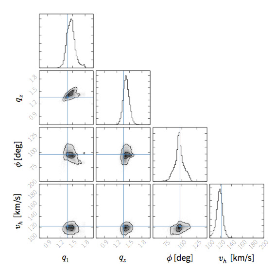Figure 3. Example using the results from the Rewinder algorithm to illustrate the power of the tidal tails as potential measures. A model galaxy containing a tidally disrupted dwarf galaxy was simulated. Four debris particles were then “observed” with errors expected for RR Lyrae stars surveyed with Spitzer (i.e., 2% distances from the mid-IR period-luminosity relation, see Madore & Freedman 2012), Gaia (i.e., very accurate proper motions) and ground-based radial velocity errors of 5 km s−1. In this case, four potential parameters (the velocity scale vh, axis ratios q1, qz and orientation φ of the dark matter halo component in which the simulation was run) were recovered with few percent accuracies on each. Reproduced from Price-Whelan et al. (2014).

¹ As discussed in Chapter 6, while there are a very limited number of potentials for which exact analytic actions are known, there has been recent progress in various approximate techniques for finding actions more generally (Sanders 2012, Bovy 2014, Sanders & Binney 2015). These advances are promising, but the extent of their effectiveness for the purposes of generating accurate models of streams in realistic triaxial potentials has yet to be fully assessed. Back.