3. USING TIDAL DEBRIS TO PROBE DARK MATTER SUBSTRUCTURE

3.1. Cosmological Context

As discussed in the Introduction to this Chapter, standard ΛCDM models of the Universe predict an order of magnitude more dark matter subhalos within the halos of typical galaxies than the number of known satellite galaxies orbiting the Milky Way (Klypin et al. 1999, Moore et al. 1999) This discrepancy can partially be explained by accounting for the incomplete sky coverage of SDSS and the distance-dependent limit on this survey's sensitivity to low-surface brightness objects (Tollerud et al. 2008, Koposov et al. 2009). Indeed, models which take this into account and consider diffuse, (i.e., undetectable) satellite galaxies can reconcile the number counts for subhalos (Bullock et al. 2010). However, when they impose the suppression of stellar populations in low mass subhalos (which have masses below 5 × 10⁸ M_⊙) the number of undetectable galaxies significantly declines and the prediction of numerous purely dark matter subhalos less massive than 5 × 10⁸ M_⊙ remains. Proof of the existence (or lack) of these “missing satellites” could provide an important constraint on the nature of dark matter, which sets the minimum scale for the formation of dark matter subhalos.

In much the same way that there is predicted to be a spectrum of dark matter subhalos in orbits about the Milky Way, we know there is a spectrum of tidal debris structures; the dominant (more extended and hotter) structures (e.g., Sgr and the Orphan Stream) arise from the infall of the larger subhalos (i.e., the ones that contain stars) while the thinner and colder streams typically come from globular clusters. All will be disturbed by subhalo-induced fluctuations in the Milky Way's potential (as first investigated by Ibata et al. (2002), Johnston, Spergel & Haydn (2002), Siegal-Gaskins & Valluri (2008)).

The key question is which streams will be most sensitive to the “missing satellites” — in particular, the multitude of low mass (M < 10⁷ M_⊙) subhalos that are predicted but whose existence has never been definitively proved. The more dominant streams have much larger cross sections and thus will encounter such subhalos more frequently, but they are also much thicker and hotter, making the effect of such individual encounters less apparent. Hence, to address this question, both the frequency of encounters of different mass subhalos as well as the size of the effect of those subhalos compared to the stream's own distribution must be accounted for (see Yoon, Johnston & Hogg 2010 for explicit calculations). For the spectrum of subhalo masses predicted by ΛCDM, it has been found that hotter stellar streams, such as Sgr, are large enough to hide the signatures of the many encounters it suffers with smaller subhalos, though the (known) subhalos containing visible satellites could have an observable effect (Johnston, Spergel & Haydn 2002). Thinner streams, such as Pal 5 and GD-1, should contain significant fluctuations in density and velocity at degree and sub-degree scales due to dozens of direct encounters with subhalos in the mass range 10⁵ – 10⁷M_⊙ over their lifetimes (Yoon, Johnston & Hogg 2010, Carlberg 2012).

Given these results, in subsequent sections we restrict our attention to the case of direct encounters of lower mass subhalos with thin streams that are typically generated by the destruction of a globular cluster.

3.2. Dark matter encounters with thin stellar streams

3.2.1 The Dynamics of Gaps in Stellar Streams

Star stream density variations on scales much smaller than the orbit of the stream are the result of encounters with perturbers (such as dark matter subhalos), the dynamics of the ejection of stars from the progenitor, and compression and expansion of a stream around an orbit.

The response of an infinitely thin stream to an encounter with a relatively low mass perturber is straightforward to calculate analytically using the impulse approximation, and the results can be generalized to streams with finite width. The results are in good agreement with numerical orbit integrations for streams with width to orbital radius ratios of 1:300, which includes the regimes of the two well studied thin streams (Pal 5 and GD-1). If a section of a stream encounters a massive satellite (e.g., the LMC), then that section of the stream will be completely pulled away and spread around the host galaxy.

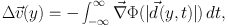
Figure 4 introduces a coordinate system for calculating the effects of subhalos passing through a stream. A perturbing mass with a spherically symmetric gravitational potential, Φ(r), induces a net velocity change, as a function of distance along the stream of:

(1)

where (y,t) is the distance along the stream from the stream crossing point at (x, y) = (0,0). Equations 1 are straightforward to numerically integrate for most radially symmetric density profiles.

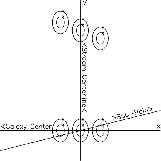Figure 4. A coordinate system to analyze the development of gaps in a stream. The stream is moving upward along the y axis. The guiding centers of three masses at different locations across the tidal stream are shown at y=0. At the top of the figure, the guiding centers of the same three masses are shown at a later time. The differential rotation of a galaxy means that the guiding centers of particles at larger radii drift backward. The width of the stream is determined by the combination of epicyclic motions and spread of guiding centers, the details of which depend on the orbit of the progenitor system (Carlberg 2013). In the text, we consider a subhalo that crosses the stream at y = 0 at t = 0. [Reproduced from Carlberg (2013).]

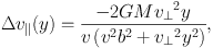
To illustrate the behavior, Carlberg (2013) analytically integrated the velocity changes of Equation 1 for a perturbing point mass, M, moving at speed (v_x, v_y), and crossing a stream that is moving along the y axis at speed V_y. The velocity of the point mass relative to the stream is defined as v_∥ = v_y − V_y (the velocity parallel to the stream), and v_⊥ = v_x (toward the stream). The distance of closest approach of the mass to the stream is the impact parameter, b. The change in the v_∥ component of the stream stars produces a change in the relative velocity of the stream and the subhalo given by:,

(2)

where v = √v_∥² + v_⊥² is the speed of the perturbing mass relative to the stream stars. This equation has been previously derived in Yoon, Johnston & Hogg (2010) with slightly different notation. For the direction of motion perpendicular to the stream, the velocity change is Δv_⊥(y) = −(v_∥ / v_⊥) Δv_∥(y). In the direction of smallest separation between the perturber and the stream (here called the z direction) the change is Δv_z(y) = (v_⊥² y / (v²b)) Δv_∥(y), which has the same sign at any location along the stream.

The effect of the perturber is to pull particles along the stream towards the crossing point, since Δv_∥(y) is positive for negative y and negative for positive y. In addition, the displacement perpendicular to the stream has the same dependence on distance along the stream and is proportional to −v_∥ / v_⊥; that is, the displacement is toward the incoming side below the crossing point (negative y) and away above it.

The velocity change was derived for a stream moving in a straight line; however, the velocity changes can be applied to a stream moving in a nearly circular orbit. For circular orbits, the particles travel along their guiding centers. The velocity changes along the stream are angular momentum changes which cause stars ahead of the crossing point (positive y) to have a reduced angular momentum and hence move to a smaller guiding center which always has a higher rate of angular rotation. Thus the stars ahead of the crossing point are pulled ahead. Similarly, the star behind the crossing point (negative y) are moved to lower angular rotation and fall behind. In this way, a gap is formed in the tidal stream.

The equations below are developed for the case of a perturber moving parallel to the orbital plane of the stream, so that the impact parameter is zero. For other orientations of the perturber, the direction of the response of the stream stars changes but the density profile of the resulting gap is essentially the same.

Stars behind the crossing point gain angular momentum and move to a larger guiding center, which has a lower rate of angular rotation, according to:

(3)

Hence, the stars begin to move apart, and a gap develops over a rotation period. The density profile of the gap can be derived from Equation 3, which gives the change in angular position of the stars with time (see Carlberg 2013). The gap starts with a size comparable to the impact parameter or scale radius of the perturbing object, and continues to grow in length with time. The material that moves out of the gap piles up on either side and creates a characteristic “double horned” density profile. The infinitely narrow stream can be broadened to a finite width by introducing a Gaussian distribution of epicycles on the stream. Epicycles are often used to describe non-circular orbits as the combination of a guiding center with a circular orbit combined with the motion of an orbiting body on an “epicycle” orbit around the guiding center. In this case, the epicycles are introduced to give the stream width; the particles will wiggle back and forth around the center of the tidal stream. The cold stream density profile of a gap is then convolved with the appropriate Gaussian distribution along the stream. Numerical integrations show good agreement with this simple theory (Figure 5). Recently Erkal & Belokurov (2014) have extended this analysis into the mildly nonlinear regime, demonstrating that the folding of the stream leads to caustics in the density profile and that the growth in the width of the stream with time slows from t to √t.

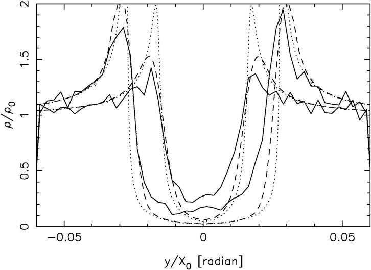Figure 5. The gap at two times (6.4 and 12.8 orbits after the encounter) in a detailed orbit integration (jagged continuous line) in a warm stream of width 0.005 relative to the orbital radius. The dotted line shows the predicted density profile for a cold stream and the dashed line is the prediction allowing for epicyclic motions. The simple theory is in good agreement with the simulation. [Reproduced from Carlberg (2013).]

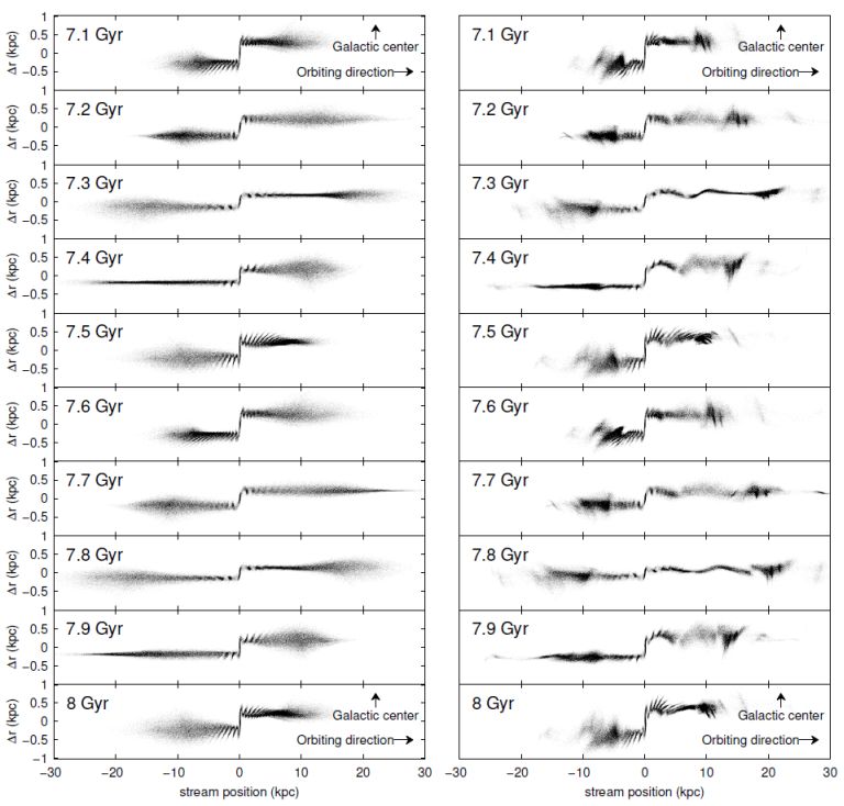Figure 6. Left panels: Simulation of a stream that develops from a globular cluster, projected onto its orbital plane, and transformed to cartesian coordinates. Δ r is the difference between the distance from the progenitor to the Galactic center and the distance from the stream debris to the Galactic center. Stream position is measured along the tidal stream. Right panels: Same as the left column, but with subhalos included in the simulation, excluding subhalos above 108 M⊙.

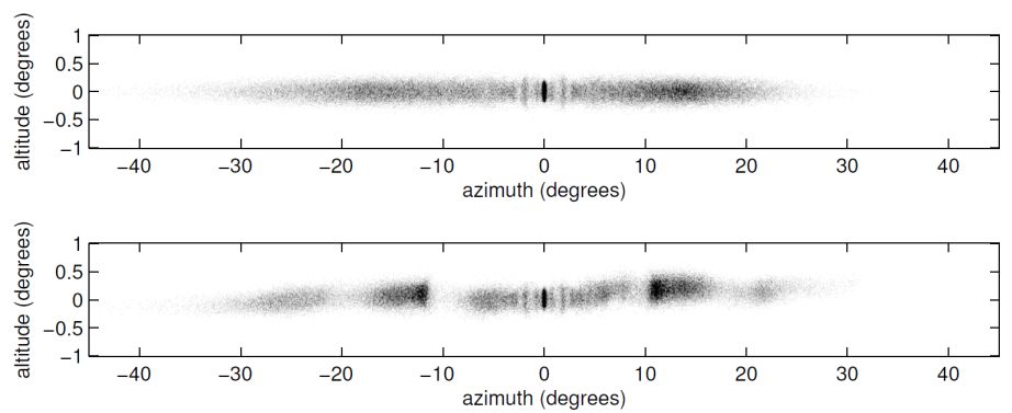Figure 7. The view from the center of the galaxy of the 7.5 Gyr timeslice of Figure 6. The top panel shows the simulated tidal stream without subhalos, and the bottom panel includes a cosmologically motivated set of subhalos in the simulation. This projection is likely closer to a typical view of a stream outside the solar circle. The youngest part of the stream, close to the progenitor, contains epicyclic oscillations which phase mix away. The stream becomes older further away and is dominated by subhalo induced gaps.

One important outcome of a number of simulations is that the range of angular momentum within the streams from a globular cluster is quite small. This implies that there is an almost unique association between time since ejection from the globular cluster into the stream, and distance from the progenitor along the stream. Furthermore, there is very little shear present at any given distance along the stream, meaning that features in the stream are not blurred out significantly with time (Bovy 2014, Carlberg 2014).

Although in principle it is possible to work out the distribution of the number of gaps of a given size in a stream, the number of effects that need to be modeled mean that it is easier to do either a partially numerical integration, or a complete simulation. The basic idea is straightforward: small sub-halos cause small gaps (which subsequently grow with time). Therefore we expect that there will be a spectrum of gap sizes rising as a power law towards smaller gaps until the spectrum rolls over because random motions in the stream blur out gaps that are smaller than about the stream width. Carlberg & Grillmair (2013) presented a semi-analytic calculation of this spectrum. Two important effects are left out of the calculation. First, the gaps will overlap, meaning that the semi-analytic calculation is an upper limit. Second, some of the gaps might not be observable given a finite number of detected stars in the stream.

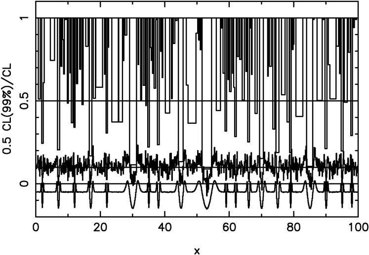Figure 8. A demonstration of the gap filter applied to artificial data with noise characteristics comparable to GD-1. The filter systematically over-estimates the number of gaps by about 44%. The filter is a well-defined approach to finding and measuring gaps, but this version is subject to (calibratable) systematic errors.

3.2.2 The cumulative effect of sub-halos

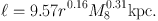
Carlberg & Grillmair (2013) refined the cold-stream analysis of Carlberg (2012) to predict that the number of gaps created per unit time per unit length in the stream (the gap creation rate, R_∪) as a function of galactocentric distance, r, in units of 30 kpc, and M₈ = M / 10⁸ M_⊙ of,

(4)

At an encounter age of around 4 Gyr, sub-halos of mass M₈ create gaps of mean length ℓ,

(5)

Eliminating M₈ between Equations 4 and 5, we find the gap creation rate as a function of gap size is:

(6)

for gaps of size ℓ, which is measured in kpc and the variable r is scaled to 30 kpc. If we evaluate this at 15 kpc for a stream of 4 Gyr age and integrate over all gap sizes larger than ℓ we find the fraction of the stream length that has gaps is

(7)

That is, for streams within about 30 kpc of the Galactic center, every position along a star stream of this age has been affected by a subhalo (Carlberg 2009). The dependence on gap size is very weak. The low mass subhalos heat the stream and to some degree frustrate and complicate the formation of subsequent small gaps. However, the stream remains intact. The larger subhalos that create gaps of several kpc in size cause sufficiently large perturbations perpendicular to the stream that it becomes possible for the orbits of stream segments to diverge, particularly if the overall potential is strongly triaxial (or more complicated) and/or time evolving.

Work has begun on the dynamical modeling of streams in realistic cosmological halos. Cooper et al. (2010) examined streams already formed within a cosmological simulation which usefully illustrate the complicated time evolution of the stream shape. However, these simulations do not have the mass resolution to follow cool streams or globular cluster dissolution. Bonaca et al. (2014) have published a realistic, but approximate, approach to following a dissolving cluster in an evolving halo. One basic outcome is that streams that orbit in the outer parts of the galaxy halo are much less disturbed than those that orbit within the much more dynamic inner parts of the galaxy halo, as expected. The buildup of the visible stellar mass which dominates the potential field of the inner galaxy has yet to be modeled.

3.2.3. Detecting Gaps in Stellar Streams

The calculations of gap shapes above usefully predict that gaps should have a double-horned profile with an integral along their length of zero, meaning the mass displaced from the gap is simply piled up on either side of the stream. Gap finding then consists of running filters of all widths along the stream to find regions where there is a good match, identified as local peaks in the filtered distribution. To quantify the statistical confidence, the same filter is run through a density distribution with the same noise properties. The resulting distribution of peaks is sorted to identify what level constitutes 99% confidence that a peak is not a false positive. Although this filtering procedure gives gap-finding a statistical foundation, the current procedures could be improved. In particular, the rate of false positives is currently about 30% of the peaks. This factor can be included as a correction, but reducing their number would be helpful. The shape of the gap filter is currently essentially an informed approximation and is not driven by the characteristics of the gaps in the data. That is, there is no current empirical approach to generate a gap spread function, comparable to the point spread function of a star that can be empirically determined in image data. Work is now beginning to undertake more extensive simulations; placing those results into a simulated sky will greatly improve the understanding of gap finding techniques.

Figure 9. A comparison of the recovered GD-1 cumulative distribution of gap sizes with the semi-analytic estimate of the expected numbers for various assumed mean stream ages.

3.3. Current observations and future prospects

Currently there are only two really well studied thin streams: the Pal 5 stream, emanating from the tidal lobes of the Pal 5 globular cluster, and the GD-1 stream, having no known progenitor.

There are three primary reasons for density variations in streams: the dynamics of mass loss from the progenitor, variations in velocity around the stream's orbit, and perturbations caused by encounters of the stream with any massive object. Massive objects range from baryonic structures to dark matter sub-halos, possibly containing visible stars or gas. The orbital effects are necessarily smooth variations around the orbit and hence on scales much larger than those which vary with the comparable size scales of the progenitors and the dark matter sub-halos of interest, which we review below.

So far streams are detected through measurements of sky density, most often in the SDSS survey where the requirement for photometric colors precise to about 10% or better limits the data to about 21-22 magnitude in the SDSS system. Reaching large numbers of stars requires getting to at least the bottom of the red giant branch and ideally to main sequence turn off stars (or beyond) at absolute magnitudes of +5 or so. The outcome is that streams tend to be found at distances in the range of 10-20 kpc in the currently available data. Even with the very good optimal weighting procedures of Rockosi et al. (2002), which dramatically reduce the weight of background stars, the summed weight of stars in the stream is typically about 10-30% of the backgrounds. To obtain a local signal-to-noise of about one usually requires binning over the entire width of narrow streams, so no information on 2D structure is available with current data. As deeper images, with more filters and eventually kinematic data become available, the local signal to noise will dramatically rise. Consequently, the currently available data is usually restricted to being a one dimensional density along the path of the stream.

Even a 60^∘ long thin stream like GD-1 is expected to have only about a dozen or so detectable gaps over its visible length. Detecting more streams, which means going to larger Galactic radii, is a key element of the future of the field. In addition, more filter bands will allow improved optimal photometric matched filtering to include metallicity information to further suppress the foreground and background stars of the same temperature and luminosity. And finally, as better kinematic data slowly become available (note that Gaia will only reach about 20th magnitude, which is the regime where streams discovered in the SDSS pick up much of their signal), the use of improved distances and velocities for each individual star will allow us to more accurately identify which stars are in the stream, and will thus improve the detail with which models can be matched to the data. Moreover, it will then be possible to use kinematic signatures of gaps (a sideways S in velocity space) to find gaps and characterize the perturbers that caused them.

There is a vast array of planned all-sky imaging and spectroscopic surveys from both the ground and space that will transform our knowledge of stellar streams over the next decade. First, we will find new streams in the southern hemisphere, links with known streams in the north, and, in both hemispheres, find streams out to about 100 kpc with higher signal-to-noise than current data. Spectra will provide astrophysical information about the nature of the stream progenitors and stream kinematics, which will be particularly powerful in combination with proper motion and distance data. The challenge will then be to make use of these data, which will be somewhat noisy by theoretical standards, to put new and interesting constraints on the nature of both the smooth large scale potential of the galaxy, and the small scale variations in the potential expected in a ΛCDM universe.

KVJ thanks her postdocs and graduate students for invaluable discussions throughout the year (Andreas Kuepper, Allyson Sheffield, Lauren Corlies, Adrian Price-Whelan, David Hendel and Sarah Pearson). Her work on this volume was supported in part by NSF grant AST-1312196. RGC thanks his graduate student Wayne Ngan and support from CIfAR and NSERC is gratefully acknowledged.