


Since the discovery of cold fronts, a large number of simulations have been performed to model their formation and evolution in merging galaxy clusters. In this review, we focus on those recent simulations which have attempted to place constraints on the detailed physical properties of the underlying plasma. A table listing the major simulations of cold fronts referenced in this paper, along with the numerical models employed and other properties, can be found in Appendix A.
We will first outline the basic physics underlying these simulations. As previously mentioned, due the fact that the electron and ion mean free paths are smaller than the length scales under consideration, the ICM is typically modeled as a thermal, magnetized plasma in the fluid approximation. However, contrary to the usual MHD ordering of scales, the Larmor radii of the particles are much smaller than their mean free paths, where the Larmor radii are on the order of npc compared to the kpc scale of the mean free path. Therefore, a given particle gyrates many times around the local magnetic field line before encountering another particle. Due to the small Larmor radii and the relative weakness of collisions, we may deduce that the perpendicular and parallel pressures of the particles and the transport coefficients of diffusive processes are anisotropic with respect to the local direction of the magnetic field line. In this situation, the anisotropy of the perpendicular and parallel pressures is produced by the conservation of the first and second adiabatic invariants of the particles.
Under these assumptions, the fluid description of the ICM can be written down in terms of the Braginskii-MHD equations (Braginskii 1965, presented here in conservative form, and in Gaussian units). The equations for conservation of mass, momentum, energy, and magnetic field are:
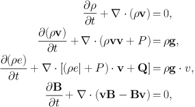 |
(3.1) (3.2) (3.3) (3.4) |
where the total (thermal and magnetic) pressure tensor in Equation 3.2 and 3.3 is
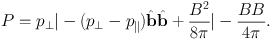 |
(3.5) |
As usual,  =
B / B is the unit vector in the direction of the local
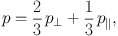
magnetic field, and the total thermal pressure satisfies
=
B / B is the unit vector in the direction of the local
magnetic field, and the total thermal pressure satisfies
 |
(3.6) |
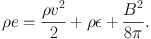
The terms B2 | / 8π and − BB / 4π in Equation 3.5 are the familiar “magnetic pressure” and “magnetic tension”, respectively. In Equation 3.3, the total energy per unit volume is
 |
(3.7) |
In these equations, ρ is the gas density, v is the fluid velocity, є is the gas thermal energy per unit volume, B is the magnetic field vector, g is the gravitational acceleration, Q is the heat flux vector, and | is the unit dyad. Generally, an adiabatic equation of state of an ideal gas p = (γ − 1)ρє with γ = 5/3 is assumed, along with equal electron and ion temperatures, and primordial abundances of H and He with trace amounts of metals, for an average molecular weight of Ā ≈ 0.6.
Most of the astrophysical literature on galaxy clusters does not present the MHD equations with a pressure anisotropy, but instead describes this effect in terms of a viscous flux. We will now show how these two descriptions are equivalent. Differences in the two components of the thermal pressure arise from the conservation of the first and second adiabatic invariants for each particle on timescales much greater than the inverse of the ion gyrofrequency, Ωg−1 (Chew et al. 1956). When the ion-ion collision frequency νii is much larger than the rates of change of all fields, an equation for the pressure anisotropy can be obtained by balancing its production by adiabatic invariance with its relaxation via collisions (cf. Schekochihin et al. 2005):
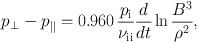 |
(3.8) |
where pi is the thermal pressure of the ions (due to their much smaller mass, the effect of the electrons on the viscosity may be neglected).
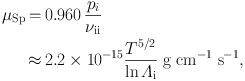
The factor in front of the time derivative on the right-hand side of Equation 3.8 is simply the dynamic viscosity coefficient for the ions, or the “Spitzer” viscosity, which is given by (Spitzer 1962, Braginskii 1965, Sarazin 1988):
 |
(3.9) |
where the temperature T is in Kelvin, νii is the ion-ion collision frequency, and lnΛi is the ion Coulomb logarithm, which is a weak function of ρ and T; for conditions in the ICM, it may be approximated as lnΛi ≈ 40. Using Equations (3.1) and (3.4) to replace the time derivatives of density and magnetic field strength with velocity gradients, Equation 3.8 may be written as
 |
(3.10) |
which, upon plugging back into Equation 3.2, shows that the effect of the pressure anisotropy manifests itself as an anisotropic viscous flux.
Next, we consider the effect of thermal conduction. Due to the effect of the small Larmor radii of the electrons, heat only flows along the field lines, and the only component of the temperature gradient which affects the heat flux is that which is parallel to the field direction:
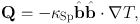 |
(3.11) |
where κSp is the familiar “Spitzer” thermal conductivity coefficient (Spitzer 1962, Braginskii 1965, Sarazin 1988):
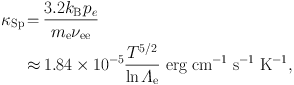 |
(3.12) |
where pe is the thermal pressure of the electrons, νee is the electron-electron collision frequency, and lnΛe is the electron Coulomb logarithm, which may also may be approximated as lnΛe ≈ 40. Due to their much larger mass, the heat flux due to ion collisions is negligible, so it is neglected.
So far, most simulations of the ICM have not worked with the full set of these equations, but rather in certain physically-motivated limits (though Dong & Stone 2009, Kunz et al. 2012, Parrish et al. 2012, Suzuki et al. 2013, and ZuHone et al. 2015a are notable exceptions). In particular, there have been two approximations of these equations in common use. In the limit that the pressure anisotropy p⊥ − p∥ is small (in other words, collisions are relatively strong and the viscosity is low), we recover standard MHD (or simply HD if it is assumed that the magnetic field can also be neglected). In this review we will describe a number of simulations that work in this MHD limit, which emphasize the effect of the magnetic field on cold fronts. Since the Prandtl number of the Spitzer description of the ICM is very small, the thermal diffusivity dominates over the momentum diffusivity:
 |
(3.13) |
Therefore, another limit of these equations considers MHD with thermal conductivity added. We will also consider a number of simulations that have operated in this limit.
A second limit of these equations that is often modeled is that in which the magnetic field is very weak and turbulent throughout the volume of the cluster. In this case, though the effects of magnetic pressure and tension are neglected, the anisotropy of the heat and momentum fluxes manifests itself as an effective suppression of the transport coefficients when averaged over a small volume, assuming the magnetic field is isotropically tangled. We may then re-write Equations 3.2 and 3.3 as:
 |
(3.14) (3.15) |
and the conductive and viscous flux terms may be written as
 |
(3.16) (3.17) |
where the “suppression factors” fc and fv account for the reduced conductivity and viscosity due to the averaging over the random direction of the magnetic field, or other microscale processes that suppress the effective conductivity and/or viscosity below the Spitzer value. This HD limit of the equations is the approximation that has been assumed in a number of simulation works, including some important ones considered in this review. Consideration of this limit is relevant, since the finite-Larmor radius effects on the transport coefficients may often only reveal themselves in a spatially averaged way due to projection effects and the finite resolution of X-ray observations.
It is also important to note that the Braginskii-MHD equations are ill-posed in situations where the absolute value of the pressure anisotropy exceeds certain bounds (on the order of the magnetic pressure), and in this regime finite-Larmor radius effects become important. We will describe these issues further and the consequences of these effects for simulations of the ICM in Section 4.1.1.
3.2. Results from Simulations of the Formation and Global Evolution of Cold Fronts
The basic physics of the formation and global evolution of cold fronts can be understood in the pure hydrodynamics framework for both the remnant core and the sloshing variety. The results of these studies, in particular their points of divergence from observed cold fronts, indicated the need for additional physics beyond HD that is discussed in subsequent sections.
Stripping of gas from one gravitational potential falling into another, usually larger, gas-filled potential has been simulated in various contexts, ranging from stripping of gas clouds inside galaxy halos (e.g., Murray et al. 1993, Pittard et al. 2010), to elliptical galaxies in clusters (e.g., Lea & De Young 1976, Takeda et al. 1984, Portnoy et al. 1993, Stevens et al. 1999, Acreman et al. 2003, Takizawa 2005, etc.) to mergers between clusters (Roettiger et al. 1997, Ricker & Sarazin 2001, Ritchie & Thomas 2002, Poole et al. 2006, Poole et al. 2007, Poole et al. 2008). Such simulations routinely produce a remnant core cold front at the upstream side of the stripped atmosphere. Strictly speaking, several of these idealized simulations do not prove that gas stripping forms an upstream cold front because they already start with a cold front, a contact discontinuity between the cooler to-be-stripped atmosphere and the hotter ambient medium. However, simulations of high mass ratio cluster mergers such as Poole et al. (2006) and ZuHone (2011) demonstrate that remnant merger core cold fronts form readily in such situations. Heinz et al. (2003) pointed out an additional effect that may help to form and maintain the upstream cold front. They suggest that the flow of ambient gas around the stripped atmosphere causes a slow forward motion of the gas inside the stripped potential, bringing cooler gas from the center of the infalling atmosphere towards the upstream edge. However, this does not seem to be a universal process and may depend on the depth and steepness infalling potential as well as on the timescale available for the stripping during the cluster infall (Roediger et al. 2015a, hereafter R15A). All purely hydrodynamical simulations of the formation of such remnant-core cold fronts that have sufficient resolution predict the growth of KHIs along the sides of the stripped atmosphere.
 |
Figure 8. Formation of a merger-remnant cold front in a purely hydrodynamic simulation from Heinz et al. (2003). Slices are of gas entropy, with velocity vectors overlaid. Note the rapid development of KHI. |
Ascasibar & Markevitch (2006, hereafter AM06) carried out simulations of sloshing cold fronts with the Gadget SPH code, and first described in great detail the formation and evolution of these features. Roediger et al. (2011) and Roediger et al. (2012b, hereafter R12) demonstrated that the positions of the sloshing cold fronts and the contrasts in density and temperature across them can be used to determine the merger history of a given cluster. In the simulations of AM06, the cold fronts which formed were stable against KHI in spite of the presence of shear flows along them, since the SPH method employed at the time was unable to resolve the KHIs. Simulations with grid codes, however, routinely predict KHIs at sloshing cold fronts. ZuHone et al. (2010) performed sloshing simulations using identical initial conditions as AM06, except that in their case the simulations were carried out using the FLASH grid-based code. Though the same cold fronts were formed in both sets of simulations, the FLASH simulations produced KHI at the interfaces (see Figure 9). KHIs also developed naturally in the sloshing simulations for the Virgo cluster and A496 (Roediger et al. 2011, R12, R13). Their appearance in synthetic X-ray observations is discussed in Section 3.4.
 |
Figure 9. Sloshing cold fronts (shown with slices of gas temperature) from an SPH simulation by AM06 (left) and a grid-based simulation of the same cluster setup by ZuHone et al. (2010) (right). The grid-based simulation resolves KHI that are unresolved by the SPH simulation. |
Many cold fronts are believed to be free of KHIs. The following sections discuss ICM plasma properties that could suppress them.
Throughout most of the volume of a galaxy cluster, the magnetic field strength is dynamically negligible. The influence of the magnetic field is typically parameterized by the plasma parameter β = pth / pB, the ratio of the thermal pressure pth and the magnetic pressure pB = B2 / 8π. Faraday rotation measurements (RM) constrain the value of β to be as low as ∼50 or as high as several hundred, with the magnetic field strength decreasing in radius from the cluster center, and turbulent on scales ranging from 100 kpc down to 100 pc, as determined from RM maps (se Carilli & Taylor 2002, Eilek & Owen 2002, Govoni et al. 2006, Laing et al. 2008, Bonafede et al. 2010, Guidetti et al. 2008, Guidetti et al. 2010, Feretti et al. 2012.
However, the existence of the discontinuous changes in density and temperature observed in cold fronts leads to the expectation that the magnetic field in these regions may not be typical of the cluster as a whole. This was first shown for the case of remnant-core cold fronts using analytic arguments by Lyutikov (2006). As a cold front moves through the magnetized medium, the field is is amplified and aligned with the cold front surface as the flow stretches and wraps or “drapes” the field lines around the interface. This effect occurs whether the cold front is moving subsonically or supersonically, so long as the velocity is super-Alfvénic, which is easily satisfied for the weak magnetic fields in the ICM. The draping layer that forms is very thin compared to the radius of curvature of the cold front, and has a magnetic pressure nearly equal to the surrounding pressure.
Using an analytical stability analysis and simulations, Dursi (2007) showed that a thin magnetized layer located at a cold front-like interface could stabilize interfaces even against long-wavelength perturbations of KHIs and Rayleigh-Taylor instabilities (RTIs). In particular, they showed that given a magnetic field layer with thickness l, to stabilize wavelengths λ ≈ 10l requires that the Alfvén speed in the layer is comparable to the relevant destabilizing velocity–namely, the shear velocity in the case of KHI. This was followed up with simulations by Dursi & Pfrommer (2008), who performed a detailed study of the propagation of cold clumps of gas through a magnetized medium. They established that the magnetic field strength in the draping layer that forms is set by a competition between the “plowing up” of field lines around the cold front and the slipping of field lines around the sides of the front. An animation showing this effect can be seen in Figure 10. Another early set of MHD simulations of the formation of remnant-core cold fronts that were explicitly used to investigate the effects of the draping layers were carried out by Asai et al. (2004, 2005, 2007, hereafter together referred to as “Asai-MHD”). These simulations used a similar setup to the simulations of Dursi & Pfrommer (2008), but also included gravity and had various initial configurations for the magnetic field lines ranging from uniform to turbulent. The Asai et al. (2004) simulations were carried out in 2D, and the Asai et al. (2005) and Asai et al. (2007) simulations were carried out in 3D.
 |
Figure 10. The draping of magnetic field lines around a cold cloud in the simulations of Dursi & Pfrommer (2008). The cutting plane is colored by magnetic energy, as are the magnetic field lines. The corresponding animation can be viewed at http://vimeo.com/160767845. |
In all of these simulations, the magnetic draping layers that form suppress KHI at the interface (see Figure 11 for examples of the temperature and magnetic field distributions from one of the Asai et al. 2007 simulations), as predicted by Lyutikov (2006). Importantly, these works showed that such layers also formed regardless of the initial field configuration, whether uniform or turbulent. They also find that the convergence of the flow behind the subcluster amplifies the field in this location as well. The Asai-MHD simulations also included anisotropic thermal conduction, which will be discussed in Section 3.5.
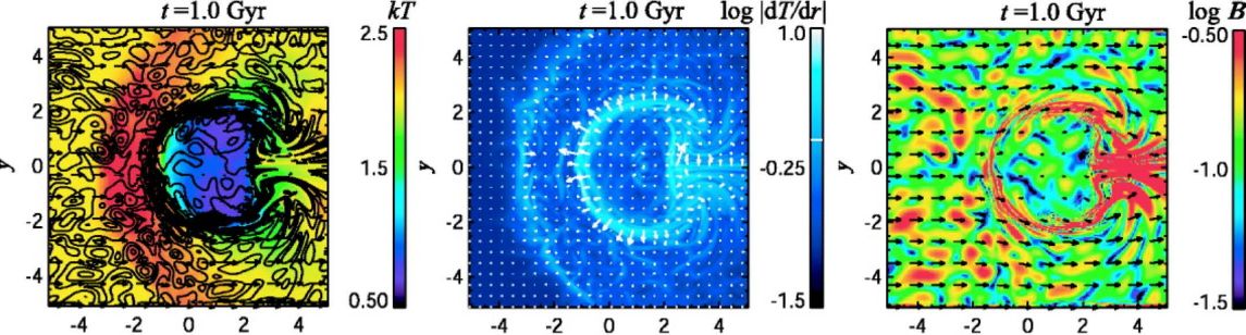 |
Figure 11. Slices through the temperature (left), temperature gradient (middle), and magnetic field strength (right) for the formation of a cold front in a magnetically turbulent medium from Asai et al. (2007). The solid curves in the left panel show the contours of the magnetic field strength. Arrows in the left and right panels show the velocity vectors, and arrows in the middle panel show the gradients of temperature. A length unit of “1” corresponds to 250 kpc. |
The MHD cluster merger simulations of Takizawa (2008) also produced magnetic draping layers at the cold front surfaces, but these simulations had low resolution and were not used to investigate the properties of cold front stability. It should also be noted that magnetic draping effects may also be responsible for the stability of AGN-blown bubbles; which has been demonstrated by a number of simulation works (Robinson et al. 2004, Jones & De Young 2005, Ruszkowski et al. 2007, Dong & Stone 2009, O’Neill et al. 2009). In particular, Ruszkowski et al. (2007) pointed out that the ability of the magnetic fields to stabilize a buoyantly rising bubble depends on the coherence length of the fields. If the latter is smaller than the bubble radius, no useful draping layer can form, and the bubble dissolves by KHIs and RTIs. The simulations of Asai et al. (2007) indicate that for remnant core cold fronts a draping layer forms quickly also for a turbulent magnetic field with a coherence length smaller than the remnant atmosphere.
Though similar magnetic field layers to the remnant-core cold fronts are also expected to appear in sloshing cold fronts, they are also somewhat different. In the remnant-core case, the movement of the cold, dense gas through the surrounding ICM builds up a layer of amplified magnetic field on the outside of the interface (Lyutikov 2006). In the case of sloshing cold fronts, in simulations we often find a velocity shear across the front surface due to the velocity difference between the fast moving cold gas beneath the front, moving tangential to the interface, and the slowly moving hot gas above the front (see also Keshet 2012). This shear amplifies the magnetic field via line freezing, d(B / ρ) / dt ≃ [(B/ρ) · ∇]u, on the inside of the interface (Keshet et al. 2010a). Figure 12 shows an animation of sloshing cold fronts using slices of gas density and magnetic field strength from an MHD simulation (ZuHone et al., in preparation).
 |
Figure 12. Slices of gas temperature (left) and magnetic field strength (right) in an MHD simulation of gas sloshing (ZuHone et al., in preparation). An animation of the development of the cold fronts and the magnetized layers over ∼2 Gyr can be found at http://vimeo.com/160771386. Along the front surfaces, the magnetic field strength is increased, and the magnetic field within the cold fronts remains high as the cold fronts expand. |
The first simulations of sloshing cold fronts to include magnetic fields were those of ZuHone et al. (2011, hereafter ZML11). They performed a parameter space exploration over the initial magnetic field configuration. The initial magnetic field was either turbulent or purely tangential, and the average field strength and its coherence length scale were varied. The former was set by enforcing the β parameter to be the same everywhere. This produces a declining magnetic field radial profile which is consistent with existing observations (Bonafede et al. 2010).
In these simulations, the shear flows initiated by the gas sloshing produce highly magnetized (low-β) layers just underneath the cold front surfaces. Figure 13 shows slices of the plasma β for the simulations with varying magnetic field strength. These layers are produced in all of the simulations, but the strength of the layer depends on the strength of the initial field. For example, the bottom-right panel of Figure 13 shows a magnetic layer in the cold front to the southwest which is nearly in equipartition with the thermal pressure, but the corresponding layers in the simulations with initial weaker field (increasing β) are not nearly as strong. Roughly, the magnetic pressure in the layers is increased by an order of magnitude over the initial field. These strongly magnetized layers are transient, only occurring directly underneath the front surface as the fronts expand. Within the increasing volume defined by the expanding fronts, the magnetic field that develops in the core behind the front is stronger than the initial field by a factor of a few. This field is typically very turbulent, except exactly below the front surface.
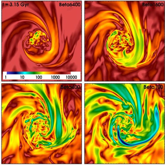 |
Figure 13. Slices through the plasma β for the simulations from ZML11 with varying initial β. Each panel is 500 kpc on a side. Major tick marks indicate 100 kpc distances. |
Figure 14 shows slices through the gas temperature for the same simulations at the same epoch. For simulations with stronger initial field, the magnetic field in the layers becomes stronger, and more capable of suppressing KHI. Figure15 shows a side-by-side animation of gas sloshing in an unmagnetized vs. a magnetized medium (ZuHone et al., in prep), showing again that the magnetic field suppresses the growth of KHI considerably compared to a case where there is no magnetization. For essentially complete suppression of KHI, the initial magnetic pressure must be at least roughly 1% of the thermal pressure, or β ≲ 100. In contrast, ZML11 did not find that the suppression of KHI has a strong dependence on the coherence length of the magnetic field fluctuations or the magnetic field geometry (whether turbulent or tangential), provided that the field strength was the same (Figure 22 of ZML11).
 |
Figure 14. Slices through the gas temperature for the simulations from ZML11 with varying initial β. Each panel is 500 kpc on a side. Major tick marks indicate 100 kpc distances. |
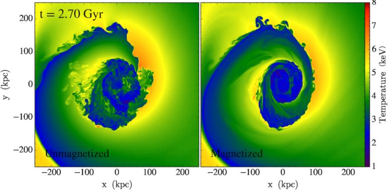 |
Figure 15. Comparison of simulations of gas sloshing with and without magnetic fields. Panels show slices of gas temperature. In the magnetized simulation, β ∼ 100. An animation of the sloshing cold fronts developing over ∼ 2 Gyr can be found at http://vimeo.com/160770528. KHI develop more readily in the unmagnetized simulation. |
However, they did find that these conclusions were somewhat dependent on resolution–for a simulation with initial β = 100 and a finest resolution of 2 kpc, KHI is highly suppressed, but for an otherwise identical simulation with a finest resolution of 1 kpc, small-wavelength KHI were able to grow (Figures 38 and 39 of ZML11). This is likely due to a confluence of two factors: the decreased numerical viscosity associated with higher spatial resolution, and the decrease in the wavelength at which KHI can be suppressed due to the thinning of the magnetized layer which occurs with decreased resolution (see Dursi 2007). Given these facts, and the uncertainties associated with the magnetic field strength in clusters, it is uncertain that magnetic fields provide the observed suppression of KHI in all clusters where such suppression is observed.
Magnetic fields may also explain the peculiar linear features seen in the observations of the Virgo cold front by Werner et al. (2016) (Figure 6). Figure 16 shows slices of density, temperature, and magnetic field strength, and residuals of surface brightness for a simulation designed to reproduce the Virgo cluster cold fronts (based on the simulations from ZuHone et al. (2015a), using the initial conditions from R12. The initial magnetic field strength for the simulation was set by β ∼ 100. The images show a region of the cluster approximately located at the same place where the observations of Werner et al. (2016) were taken. They show narrow, quasi-linear, dense, cold features, which correlate to narrow channels of weak magnetic field in between wide bands of strong magnetic field which are less dense and hotter. The dense features produce surface brightness features similar to those seen in Figure 6.
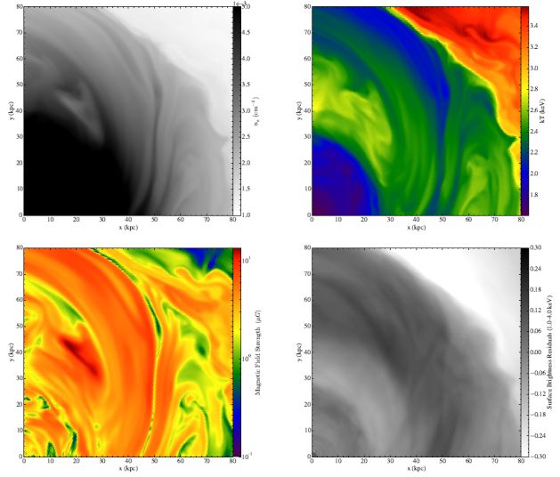 |
Figure 16. Sloshing in a Virgo-like simulated cluster from Werner et al. (2016). Top left: Slice through the center plane of electron density. Top right: Slice of gas temperature. Bottom left: Slice of magnetic field strength. Bottom right: Projected surface brightness residuals. |
Since the magnetic field in the simulation is turbulent before the sloshing begins, the local magnetic field strength will vary from place to place. When the sloshing motions begin, the field is stretched and amplified in the direction of the sloshing, which erases much of the small-scale structure in the field. However, we may expect that perpendicular to the direction of motion, some memory of the variations in magnetic field strength will be preserved. Since the simulations demonstrate that the final amplified field strength does depend to some extent on the initial field strength, these variations will produce regions of slightly weaker magnetic field sandwiched between regions of stronger field. The total pressure across these bands (magnetic and thermal) will be continuous.
The narrow regions of slightly weaker field are correlated with regions of higher density and lower temperature compared to the surrounding regions with higher magnetic field strength. The anticorrelation between density and temperature is somewhat peculiar, as the simulations exhibiting these features are adiabatic (without sources of heating or cooling), and for an individual fluid element the entropy should be constant. This implies that a decrease in the gas thermal pressure due to an increase the magnetic pressure in the wide bands should correspond to a decrease in both the gas density and temperature in these bands, yet the temperature is higher. This may be explained by low-entropy, low-temperature, high-density gas being advected from the cluster center to larger radii by the sloshing, but it is not completely clear why such gas should be associated with regions of low magnetic field strength. In real clusters, the density enhancement and temperature decrement will be enhanced by gas cooling. A more careful investigation of this phenomenon from simulations is required.
3.4. Cold Fronts and Viscosity
Small-scale KHIs will be suppressed if the shear velocity across the interface does not change discontinuously, but is smoothed over a certain thickness ± d. In this case, KHIs of length scale ≲ 10d are suppressed (Chandrasekhar 1961, Section 102). In a viscous fluid, momentum diffusion across a shear flow interface will establish exactly such a smoothed out shear flow layer. Thus, we can naturally expect that with increasing viscosity KHIs are suppressed at ever larger length scales. Assuming an isotropic viscosity, Roediger et al. (2013b) showed that the suppression of KHIs occurs roughly at Reynolds numbers Re = LU / ν smaller than 30 to 100, where L is the length scale of the KHI, U the shear velocity, and ν = µ / ρ is the kinematic viscosity. The detailed value of the critical Reynolds number depends on the nature of viscosity (e.g., constant versus temperature dependent ν) and density contrast across the shear interface.
At full Spitzer viscosity (Equation 3.9), the critical Reynolds number for suppressing KHIs is easily reached for both remnant core and sloshing cold fronts. Furthermore, a sufficient ICM viscosity prevents the mixing of gas stripped from the infalling subcluster or galaxy with the ambient ICM in the wake (Roediger et al. 2015b, hereafter R15B). Recent deep Chandra and XMM-Newton observations resolve the structure of the cold fronts and of galaxy or subcluster wakes. However, the interpretation of the observations on their own is not straightforward because the appearance of individual objects depends on several other parameters such as the infall and/or merger history, viewing geometry, initial gas contents, or internal perturbations due to, e.g., AGN activity.
R15A and R15B simulated the infall of the elliptical galaxy M89 into the Virgo cluster and followed the progressive gas stripping process as the galaxy is crossing its host cluster. The authors showed that progressive gas stripping of a galaxy or subcluster leads to the formation of a “remnant tail” of the atmosphere (Figure 17). Gas from the galaxy’s atmosphere is removed predominantly upstream and from its sides, but the downstream part of the atmosphere is shielded from the ICM head wind (see animation in Figure 17). Consequently, the stripped atmosphere develops a head-tail structure, where the tail is simply the unstripped downstream atmosphere. Making the analogy to the flow around a blunt body, the wake of the galaxy starts only downstream of the remnant tail. These global flow patterns, i.e., the upstream edge or cold front of the remnant core, its remnant tail, and the downstream wake in the ICM are independent of viscosity.
 |
Figure 17. Snapshots from simulations of progressive gas-stripping of an elliptical galaxy, from R15A and R15B. The two top panels and the associated animation found at http://vimeo.com/160773185 show density slices through the stripped galaxy for inviscid stripping and with a viscosity of 0.1 of the Spitzer level. During the infall into the host cluster, characteristic flow regions develop, which are labelled in the bottom panel. A remnant-core cold front exists at the upstream side, stretching around to the sides of the atmosphere. Here the interface between the galactic gas and the ICM becomes KHI unstable at sufficiently low viscosity. The downstream atmosphere is shielded from the ambient flow for a long time and takes the appearance of a remnant tail. Only in the wake can stripped gas mix with the ambient gas, unless the mixing is suppressed by viscosity. |
R15B focused on observable signatures of an isotropic but Spitzer-like temperature dependent viscosity (Figure 18). In inviscid stripping, KHIs at the sides of the remnant atmosphere take the shape of horns or wings that are observable in X-ray images, and mixing of stripped colder galactic gas leads to fainter, warmer wakes. Interestingly, already at a level of 1/10 the Spitzer viscosity, KHIs are suppressed, horns or wings at the sides of the remnant core are absent, and the stripped-off colder and denser galactic gas leads to bright, cool, wakes far behind the galaxy, implying that the viscosity is low in systems such as M89 which possess evidence of “horned” cold fronts (Figure 18).
 |
Figure 18. Chandra X-ray image of the stripped elliptical galaxy M89 in the Virgo cluster (left), compared to mock X-ray images of inviscid and a viscous stripping simulations for the same galaxy (middle and right panels). The observation and simulations clearly show the remnant-core cold front, labelled “upstream edge” here. Comparing the simulations and the observations identifies the observed near tail of M89 as the remnant tail, and its wake is only found at the edge of the observed field of view. In the inviscid simulation, KHIs peel off galactic gas from the sides of the remnant core. If the Virgo ICM has a viscosity roughly 0.1 of the Spitzer viscosity, KHIs at the sides of M89 would be suppressed, and it should have a cold bright wake out to 10 times the remnant-core radius downstream of the galaxy. Reproduced from R15B. |
Suzuki et al. (2013, hereafter S13) carried out the first investigation of remnant-core cold front evolution under the influence of an anisotropic (Braginskii) viscosity. They used weak magnetic fields so that their effect on KHI suppression would be negligible. The magnetic fields were uniform in direction, oriented either perpendicular to the axis of motion of the cold front, or inclined by a 45∘ angle. They showed that anisotropic viscosity is not as efficient as an isotropic viscosity at suppressing KHIs because the damping effect of viscosity is reduced by the dependence on the field line direction (see Figure 19). In the plane parallel to the initial field line direction, KHI grows very fast, since the field lines are perpendicular to the velocity gradient at the interface. Conversely, in the plane perpendicular to the initial field line direction, the growth rate of KHI was somewhat reduced, due to the fact that the field line had components parallel to the velocity gradient. A similar dependence on the initial field direction on the growth of KHI at the surfaces of AGN-blown bubbles was found by Dong & Stone (2009), who also included Braginskii viscosity in their simulations. This points to the need for future simulations to include more realistic magnetic field configurations.
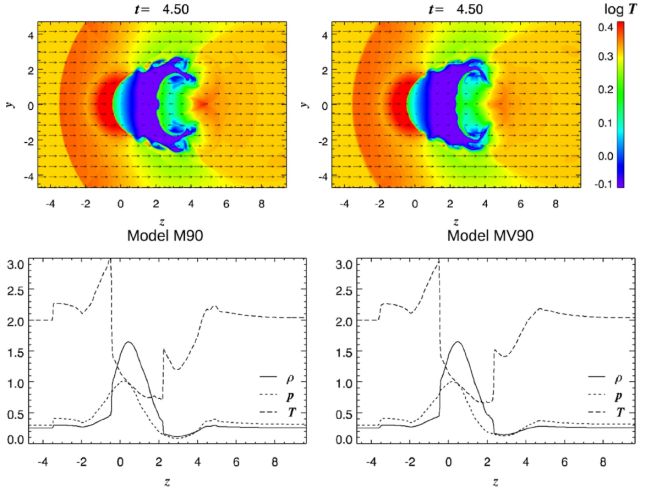 |
Figure 19. The effects of Braginskii viscosity on remnant-core cold fronts, from S13. Top panels: Slices through the gas temperature in the y − z plane from the inviscid (left) and Braginskii viscosity (right) simulations. In these units, 1 = 250 kpc. Bottom panels: Profiles of the gas density and temperature across the cold front interface, from the inviscid (left) and Braginskii viscosity (right) simulations. The cold front interface is located at z ≈ − 0.5 ( − 125 kpc). The growth of KHI in both simulations is similar, demonstrating that in this scenario Braginskii viscosity has only a marginal effect on suppressing KHI. |
The first simulation of sloshing cold fronts with an isotropic viscosity was carried out by ZuHone et al. (2010), who studied how sloshing motions in a galaxy cluster provide a source of heat to offset cooling via mixing of higher-entropy gas from larger radii with the lower-entropy gas from the core. They compared simulations without viscosity and with a constant kinematic viscosity which roughly corresponded to the Spitzer value in the core region. They found that gas mixing is very efficient if the ICM is inviscid, whereas it is negligible if the plasma is viscous. They noted that the viscosity greatly suppressed KHIs along the cold fronts.
R13 showed that the presence of KHIs at sloshing cold fronts leads to characteristic observable signatures such as a ragged appearance of the surface brightness edge and a multi-step structure of the cold front in surface brightness profiles (Figure 20). In contrast, suppressing KHIs with an isotropic, temperature-dependent, Spitzer-like viscosity with a suppression factor of fv ∼ 0.1, led to smooth sloshing cold fronts and a clean, single step edge in surface brightness profiles. Furthermore, the region below the cold fronts shows much stronger surface brightness fluctuations in the inviscid case than in the viscous one. The deep Virgo observations of Werner et al. (2016) show both surface brightness fluctuations below the cold front and a multi-step structure of the cold front itself, which may indicate the presence of KHIs and a strongly suppressed ICM viscosity in the Virgo cluster. Distorted or “ragged” sloshing cold fronts have also been identified in the merging groups NGC 7618 / UGC 12491 (Roediger et al. 2012a, Figure 7) and in A496 (Dupke et al. 2007, R12).
 |
Figure 20. Snapshot from a simulation of inviscid and viscid sloshing in Virgo cluster, from R13. An animation of the middle two panels may be found at http://vimeo.com/160772084. The middle row shows temperature slices through the cluster center in the orbital plane of the perturber. A viscosity at 0.1 of the Spitzer level erases pre-existing KHIs along the northern front, which continued to grow and form in the inviscid run. The top-right panel shows a mock X-ray image of the inviscid sloshing, zoomed in on the northern cold front. In X-ray images, KHIs appear as multiple edges and give the cold front a ragged appearance. The multiple edges also appear in narrow-wedge surface brightness profiles across the cold front (three edges are marked in the profile in the bottom-left panel). At a sufficient viscosity, however, the cold front appears as a single edge in the surface brightness profile (bottom-right). |
The first simulations of sloshing cold fronts to employ anisotropic viscosity were those of ZuHone et al. (2015a, hereafter Z15). They compared magnetized simulations with anisotropic viscosity to those with isotropic viscosity with various suppression factors fv. Similar to S13, they used weak magnetic fields (with β ∼ 1000) to isolate the effect of viscosity on KHI. Using synthetic X-ray observations, they found that anisotropic viscosity is capable of suppressing KHI at cold front surfaces to a degree that is qualitatively similar to an isotropic viscosity with a Spitzer fraction of fv = 0.1 (see Figures 21 and 22). They also compared simulations with isotropic viscosity with and without magnetic fields, and noted that even their weak seed field has effects on cold front stability that can yield observational consequences. This demonstrates that it will be essential for future studies to consider the effects of viscosity and magnetic fields together.
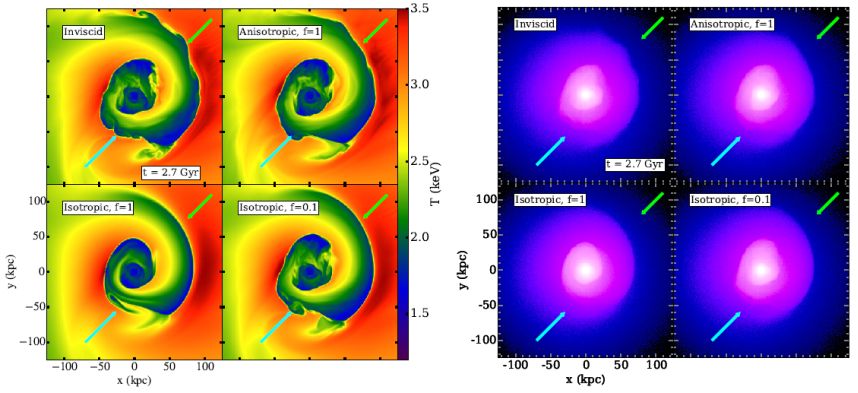 |
Figure 21. Simulations of the Virgo cold fronts with different prescriptions for viscosity, including anisotropic (Braginskii) viscosity. From top-left counterclockwise, simulations are: invsicid, Spitzer anisotropic viscosity, Spitzer isotropic viscosity, 1/10 Spitzer isotropic viscosity. Left panel: Slices through the gas temperature in keV. Right panel: Simulated 300 ks Chandra observations. Cold fronts with an appearance that has been visibly modified by viscosity are marked with arrows; for a closeup of the NW cold front see Figure 22. |
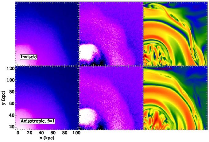 |
Figure 22. Close-up of the NW cold front in Figure 21 for simulations with inviscid and anisotropic (Braginskii) viscosity. The top panels show the invsicid simulation, whereas the bottom panels show the anisotropic viscosity simulation. From left to right, the panels show the simulated 300 ks exposure, simulated 300 ks residuals, and slice through the magnetic field strength. In the inviscid simulation, KHI distort the cold front and tangle the magnetic field lines. |
3.5. Cold Fronts and Thermal Conductivity
Due to the small electron Larmor radius, thermal conduction in the ICM should be greatly reduced perpendicular to magnetic fields. Given that magnetic fields readily align with cold fronts, we expect thermal conduction across cold fronts to be greatly reduced. Xiang et al. (2007) used pure-HD simulations of remnant-core cold front formation with isotropic thermal conduction and various suppression factors for the thermal conductivity to show that to reproduce the width of the cold front in A3667 the heat flux across the interface must be suppressed by a factor of ∼67. They also found that the thickness of the diffusive layer near the stagnation point of the cold front does not depend on the distance along the front from this point, implying that the front does not widen with distance from this point.
The previously described Asai-MHD simulations were the first to investigate the effects of anisotropic thermal conduction and magnetic fields on a remnant-core cold front. These simulations demonstrated that sufficient magnetic draping would occur around the developing cold front to suppress thermal conduction strongly enough that a sharp cold front edge could be maintained for timescales much longer than that required to smear out the cold front interface by uninhibited conduction, regardless of whether or not the initial magnetic field was uniform or turbulent. Figure 23 shows profiles of gas density, temperature, and pressure across the cold front for models with anisotropic and isotropic thermal conduction, where in the former case the cold front is shielded from conduction by the magnetic field, but in the unmagnetized latter case conduction has completely smoothed out the front surface.
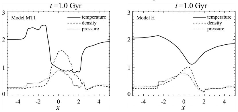 |
Figure 23. Profiles of the gas density, temperature, and pressure across the cold front interface from the simulations of Asai et al. (2007). Left panel: Profiles from the magnetically turbulent simulation with anisotropic thermal conduction. Right panel: Profiles from the unmagnetized simulation with isotropic thermal conduction. The cold front interface that is preserved by the magnetic field layer at x ≈ − 1 ( − 250 kpc) in the left panel are wiped out by conduction in the right panel. |
S13 also claimed to find that the magnetic field layer also suppressed conduction across the cold front interface for their nearly identical setup, though they noted that some smoothing out of the temperature discontinuity occurred at early times before the magnetic draping layer was able to develop. The top panels of Figure 24 show slices through the gas temperature of their magnetized simulations with anisotropic thermal conduction (with and without Braginskii viscosity). The interface does not appear quite as sharp as in their non-conductive simulations (see Figure 19). The bottom panels of Figure 24 highlight this fact in more detail, showing the profiles of density and temperature across the cold front surface at z ≈ − 0.5.
 |
Figure 24. The effects of anisotropic thermal conduction and viscosity on remnant-core cold fronts, from S13. Top panels: Slices through the gas temperature in the y − z plane from the inviscid (left) and Braginskii viscosity (right) simulations. In these units, 1 = 250 kpc. Bottom panels: Profiles of the gas density and temperature across the cold front interface, from the inviscid (left) and Braginskii viscosity (right) simulations. The density and temperature jump across the cold front interface at z ≈ − 0.5 ( − 125 kpc) appears to be smeared out by conduction, regardless of the presence or absence of Braginskii viscosity (compare with the sharp jumps in the bottom panels of Figure 19). |
ZuHone et al. (2013, hereafter Z13) were the first to carry out simulations of the formation of sloshing cold fronts in the ICM with magnetic fields and anisotropic thermal conduction. They used the same set of cluster initial conditions as ZML11, performing simulations with different thermal conductivities and magnetic field geometries, with the initial magnetic field strength set by enforcing that β = 400 everywhere. The two most important cases were a simulation with full Spitzer conduction along the field lines, and an otherwise identical simulation with 1/10th Spitzer conduction along the field lines, modeling a situation where thermal conduction is suppressed along the field line, by strong curvature of the field lines, stochastic magnetic mirrors, or microscale plasma effects (Chandran et al. 1999, Malyshkin & Kulsrud 2001, Narayan & Medvedev 2001, Schekochihin et al. 2008, also see Section 4.1.1 and references therein).
These simulations revealed an unexpected result: despite the presence of magnetic field layers, thermal conductivity was able to smear out the front surfaces to a certain degree. Figure 25 shows slices of temperature through the midplane of the sloshing cold fronts (top panels), along with profiles taken across the cold fronts in particular places (shown in the bottom panels, marked by black lines in the top panels). In the case of full anisotropic Spitzer conduction (top-right panel), the temperature jumps have been smeared out and the interior of the cold fronts have considerably higher temperature than the case of no conductivity. In the simulation with 1/10th Spitzer conduction (top-middle panel), the temperature jumps are essentially identical to those of the case without conduction. Figure 26 shows that thermal conductivity would have a significant effect on the appearance of cold fronts as seen in X-rays–full Spitzer conduction, even when restricted to the field lines, smears out the interface to such a degree that the cold fronts are essentially eliminated, as shown in Figure 26. For 1/10 Spitzer conduction, the cold fronts appear roughly the same as in the case without conduction.
 |
Figure 25. The effect of anisotropic thermal conduction on sloshing cold fronts (reproduced from Z13). Top panels: Slices of gas temperature through the center of the domain in the x − y plane from the simulations of Z13 at the epoch t = 3.25 Gyr. Each panel is 500 kpc on a side. Black lines indicate the locations of profiles taken across the cold fronts. Bottom panels: Profiles of the gas temperature taken across the lines shown in the top panels. |
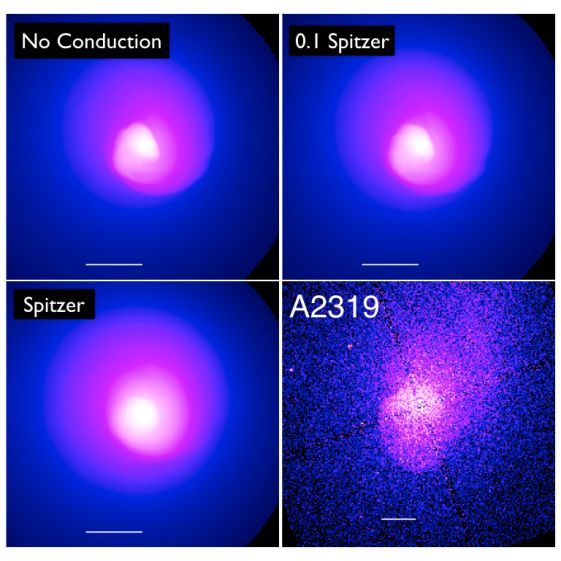 |
Figure 26. Projected X-ray emission along the z-axis of the simulation domain for the simulations from Z13 with a Chandra X-ray image of A2319 included for comparison. White bars indicate 100 kpc distances. Conduction smooths out the surface brightness jumps, making them barely discernable in comparison to the sharp jumps in emission seen in A2319. |
These results are in conflict with the initial expectation that a magnetic layer completely protects the cold front from heat conduction. Not surprisingly, the devil is in the details–the full simulations reveal two reasons why the simple picture, drawn from analytic considerations, breaks down. First, although the magnetic field is stretched tangential to the front surface by the shear flow, KHI may develop rapidly along parts of the front, tangling the field lines at the interface once again, allowing some heat to diffuse between the hot and cold phases (c.f. Figure 8 of Z13). This effect is also seen in the plane-parallel simulations of Lecoanet et al. (2012), which showed that perturbations in the magnetic field direction across an interface similar to a cold front can cause a similar smearing of the interface. Only in a scenario where the amplified magnetic field were strong enough to prevent KHI completely would this effect be absent. Secondly, the three-dimensional nature of the problem and the geometry of the cold fronts leave the cold gas underneath the front magnetically connected to hot gas above the front and perpendicular to the sloshing plane, providing yet another avenue for the transfer of thermal energy (c.f. Figures 9 and 10 of Z13). We will discuss the discrepancies between the different simulations of cold fronts with anisotropic thermal conduction in Section 4.1.3.
In the previously described work by Z15, simulations with anisotropic thermal conduction were also included, with and without Braginskii viscosity. Regardless of whether or not the ICM is viscous, the results from these simulations are the same as in Z13: anisotropic thermal conduction smears out cold fronts to such a degree that they would be unobservable, even by Chandra (see Figure 27). This implies that these constraints on thermal conduction may apply generally to clusters, as the cluster model resembling the Virgo cluster from ZuHone et al. (2015a) has a much colder average temperature than the more massive cluster model from Z13, and hence much weaker thermal conductivity, due to the strong dependence of the latter on the temperature (∝ T5/2).
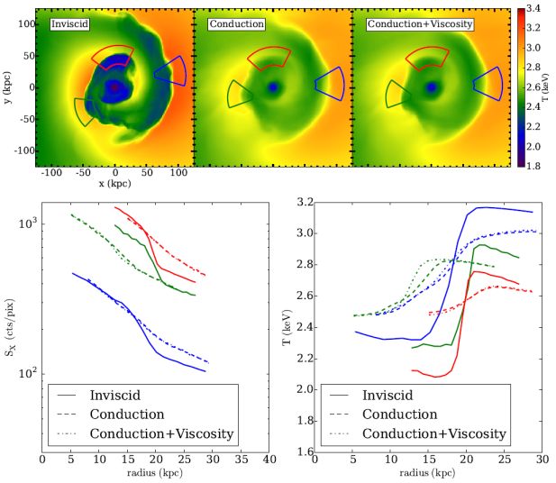 |
Figure 27. The effect of anisotropic thermal conduction on a simulated cluster similar to Virgo, from ZuHone et al. (2015a). Top panels: projected spectroscopic temperature for three different models. Colored regions show the locations of profiles in the bottom panel. Bottom panel: Profiles of surface brightness and projected temperature across the cold front surfaces at the locations given by the regions in the top panel. |