2. SUPERVISED LEARNING

Supervised machine learning algorithms are used to learn a relationship between a set of measurements and a target variable using a set of provided examples. Once obtained, the relationship can be used to predict the target variable of previously-unseen data. The main difference between traditional model fitting techniques and supervised learning algorithms is that in traditional model fitting the model is predefined, while supervised learning algorithms construct the model according to the input dataset. Supervised learning algorithms can, by construction, describe very complex non-linear relations between the set of measurements and the target variable, and can therefore be superior to traditional algorithms that are based on fitting of predefined models.

In machine learning terminology, the dataset consists of objects, and each object has measured features and a target variable. In Astronomy, the objects are usually physical entities such as stars or galaxies, and their features are measured properties, such as spectra or light-curves, or various higher-level quantities derived from observations, such as a variability period or stellar mass. The type of target variable depends on the particular task. In a classification task, the target variables are discrete (often called labels), for example, classification of spectra into stars or quasars. In a regression task, the target variable is continuous, for example, redshift estimation using photometric measurements.

Supervised learning algorithms often have model parameters that are estimated from the data. These parameters are part of the model that is learned from the data, are often saved as part of the learned model, and are required by the model when making predictions. Examples of model parameters include: support vectors in Support Vector Machines, splitting features and thresholds in Decision Trees and Random Forest, and weights of Artificial Neural Networks. In addition, supervised learning algorithms often have model hyper-parameters, which are external to the model and whose values and are often set using different heuristics. Examples of model hyper-parameters include: the kernel shape in Support Vector Machines, the number of trees in Random Forests, and the number of hidden layers in Artificial Neural Networks.

The application of supervised learning algorithms is usually divided into three stages. In the training stage, the model hyper-parameters are set, and the model and the model parameters are learned from a subset of the input dataset, called the training set. In the validation stage, the model hyper-parameters are optimized according to some predefined cost function, often using a different subset of the input dataset, called the validation set. During the validation stage, the model training is carried out iteratively for many different choices of hyper-parameters, and the hyper-parameters that result in the best performance on the validation set are chosen. Finally, in the test stage, the trained model is used to predict the target variable of a different subset of the input dataset, called the test set. The latter stage is necessary in order to assess the performance of the trained model on a previously-unseen dataset, i.e., a subset of the input data that was not used during the training and validation stages, and can be used to compare different supervised learning algorithms. Once these stages are completed, the model can be used to predict the target variable of new, previously-unseen datasets.

This section provides some basic principles of supervised machine learning, and presents several popular algorithms used in Astronomy. For a detailed review on the subject, see Biehl (2019). The section starts by describing the cost functions that are usually used to optimize model hyper-parameters, assess the performance of the final model, and compare different supervised learning algorithms (section 2.1). Then, section 2.2 gives additional details on the input dataset, in particular its partition to training, validation, and test sets, feature selection and normalization, and imbalanced datasets. Finally, three popular algorithms are presented: Support Vector Machine (section 2.3), Decision Trees and Random Forest (section 2.4), and shallow Artificial Neural Networks (section 2.5).

There are different evaluation metrics one can use to optimize supervised learning algorithms. Evaluation metrics are used to optimize the model hyper-parameters, to assess the performance of the final model, to select optimal subset of features, and to compare between different supervised learning algorithms. The evaluation metrics are computed during the validation and the test stages, where the trained model is applied to a previously-unseen subset of the input dataset, and the target variable predicted by the model is compared to the target variable provided in the input data.

In regression tasks, where the target variable is continuous, the common metrics for evaluating the predictions of the model are the Mean Absolute Error (MAE) and the Mean Squared Error (MSE). The MAE is equal to 1/n ∑_i=1ⁿ| y_i − ŷ_i |, where n is the number of objects in the validation or test set, ŷ_i is the target variable predicted by the model, and y_i is the target variable provided in the input data. The MSE is equal to 1/n ∑_i=1ⁿ( y_i − ŷ_i )². The MSE has the disadvantage of heavily weighting outliers, since it squares each term in the sum, giving outliers a larger weight. When outlier weighting is undesirable, it is better to use the MAE instead. Finally, it is worth noting additional metrics used in the literature, for example, the Normalized Median Absolute Deviation, the Continuous Rank Probability Score, and the Probability Integral Transform (see e.g., D'Isanto & Polsterer 2018; D'Isanto et al. 2018).

In classification tasks, where the target variable is discrete, the common evaluation metrics are the Classification Accuracy, the Confusion Matrix, and the Area Under ROC Curve. Classification accuracy is the ratio of the number of correct predictions (i.e., the class predicted by the model is similar to the class provided in the input dataset) to the total number of predictions made. This value is obviously bound between 0 and 1. The accuracy should be used when the number of objects in each class is roughly similar, and when all predictions and prediction errors are equally important. Confusion matrices are used in classification tasks with more than two classes. Figure 1 shows an example of a confusion matrix, taken from Mahabal et al. (2017), who trained a supervised learning model to distinguish between 7 classes of variable stars. Each row and column in the matrix represents a particular class of objects, and the matrix shows the number of objects in each class versus the number of objects predicted by the model to belong to a particular class. In the best-case scenario, we expect the confusion matrix to be purely diagonal, with non-zero elements on the diagonal, and zero elements otherwise. Furthermore, similarly to the accuracy, one can normalize the confusion matrix to show values that range from 0 to 1, thus removing the dependence on the initial number of objects in each class.

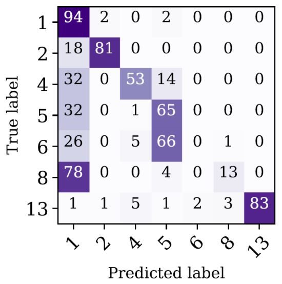Figure 1. Example of a confusion matrix taken from Mahabal et al. (2017), who trained a deep learning model to distinguish between 7 classes of variable stars, marked by 1, 2, 4, 5, 6, 8, and 13 in the diagram. The confusion matrix shows the number of objects in each class versus the number of objects predicted by the model to belong to a particular class. In the best-case scenario, the confusion matrix will contain non-zero elements only in its diagonal, and zero elements otherwise.

Finally, the receiver operating characteristic curve (ROC curve) is a useful visualization tool of a supervised algorithm performance in a binary classification task. Figure 2 shows an illustration of an ROC curve, where the True Positive Rate is plotted against the False Positive Rate. The true positive rate represents the number of "true" events that are correctly identified by the algorithm, divided by the total number of "true" events in the input dataset. The false positive rate represents the number of "false" events that were wrongly classified as "true" events divided by the total number of "false" events. For example, if we are interested in detecting gravitational lenses in galaxy images, "true" events are images with gravitational lenses, and "false" events are images without gravitational lenses. In the best-case scenario, we expect the true positive rate to be 1, and the false positive rate to be 0. The ROC curve diagram is generated by varying the model hyper-parameters, and plotting the true positive rate versus the false positive rate obtained for the validation set (the continuous ROC curves presented in Figure 2 are produced by varying the classification/detection threshold of a particular algorithm. This threshold can be considered as a model hyper-parameter). Furthermore, the diagram can be used to compare the performance of different supervised learning algorithms, by selecting the algorithm with the maximal area under the curve. For example, in Figure 2, model 1 outperforms model 2 for any choice of hyper-parameters. Finally, depending on the task, one can decide to optimize differently. For some tasks one cannot tolerate false negatives (e.g., scanning for explosives in luggage), while for others the total number of errors is more important.

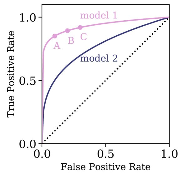Figure 2. An illustration of an ROC curve, where the true positive rate is plotted against the false positive rate. In the best-case scenario, we expect the true positive rate to be 1, and the false positive rate to be 0. The black line represents the resulting ROC curve for random assignment of classes, which is the worst-case scenario. The diagram is populated by varying the model hyper-parameters and plotting the true positive rate versus the false positive rate obtained for the validation set. The pink curve represents the ROC curve of model 1, where A, B, and C represent three particular choices of hyper-parameter value. The purple curve represents the ROC curve of model 2. The area under the ROC curve can be used to select the optimal model, which, in this case, is model 1.

2.2. Input Dataset

The input to any supervised learning algorithm consists of a set of objects with measured features, and a target variable which can be either continuous or discrete. As noted in the introduction to this section, the input dataset is divided into three sets, the training, validation, and test sets. The model is initially fit to the training set. Then, the model is applied to the validation set. The validation set provides an unbiased evaluation of the model performance while tuning the model’s hyper-parameters. Validation sets are also used for regularization and to avoid overfitting, with the common practice of stopping the training process when the error on the validation dataset increases. Finally, the test set is used to provide an unbiased evaluation of the final model, and can be used to compare between different supervised learning algorithms. To perform a truly unbiased evaluation of the model performance, the training, validation, and test sets should be mutually exclusive.

The dataset splitting ratios depend on the dataset size and on the algorithm one trains. Some algorithms require a substantial amount of data to train on, forcing one to enlarge the training set at the expense of the others. Algorithms with a few hyper-parameters, which are easily validated and tuned, require small validation sets, whereas models with many hyper-parameters might require larger validation sets. In addition, in Cross Validation the dataset can be repeatedly split into training and validation sets, for example, by randomly selecting objects from a predefined set, and the model is then iteratively trained and validated on these different sets (see e.g., Miller et al. 2017). There are different splitting methods that are implemented in python and are publicly available in the scikit-learn library ².

The performance of all supervised learning algorithms strongly depends on the input dataset, and in particular on the features that are selected to form the dataset. Most supervised learning algorithms are not constructed to work with hundreds or thousands of features, making feature selection a key part of the applied machine learning process. Feature selection can be done manually by an expert in the field, by defining features that are most probably relevant for the task at hand. There are various alternative ways to select an optimal set of features without domain knowledge, including filter methods, wrapper methods, and embedded methods. Filter methods assign a statistical score to each feature, and features are selected or removed according to this score. In wrapper methods, different combinations of features are prepared, and the combination that results in the best accuracy is selected. Embedded methods learn which features best contribute to the accuracy of the model during the model construction (see also Donalek et al. 2013; D'Isanto et al. 2016, 2018). Some to these methods are included in the scikit-learn library ³. Finally, a pertinent note on deep learning, in particular Convolutional Neural Networks. The structure of these networks allows them to take raw data as an input (e.g., spectra, light-curves, and images), and perform efficient feature extraction during the training process. Thus, using such models, there is usually no need to perform feature selection prior to the training stage.

Feature scaling is an additional key part of the data preparation process. While some algorithms do not require any feature scaling prior to training (e.g., Decision Trees and Random Forest), the performance of other algorithms strongly depends on it, and it is advised to apply some feature scaling prior to their training (e.g., for Support Vector Machine). There are various ways to scale the features in the initial dataset, including standardization, mean normalization, min-max scaling, and application of dimensionality reduction algorithms to the initial dataset. These will not be further discussed in this document, however, many feature scaling methods are available in scikit-learn ⁴.

Finally, it is worth noting the topic of imbalanced datasets. Imbalanced data typically refers to the problem of a classification task where the classes are not equally represented. During training, many supervised learning algorithms assign equal weights to all the objects in the sample, resulting in a good performance on the larger class, and worse performance on the smaller class. In addition, the regular accuracy cannot be used to evaluate the resulting model. Assume for example that we are interested in detecting gravitational lenses, and our dataset contains 100 000 images of galaxies, out of which 100 images show evidence of lensing. For such a dataset, an algorithm that classifies all objects as "not lens", regardless of the input features, will have an accuracy of 0.999. There are several methods to train and evaluate supervised learning algorithms in the presence of imbalanced datasets. One could apply different weights to different classes of objects during the training process, or undersample the larger class, or oversample the smaller class of objects. These, and additional methods, are available in scikit-learn. Instead of the classification accuracy, one can use the ROC curve (figure 2), and select the hyper-parameters that result in the desired true positive versus false negative rates.

2.3. Support Vector Machine

One of the most popular supervised learning algorithms is Support Vector Machine (SVM), which has been applied in Astronomy for a variety of tasks (e.g., Qu et al. 2003; Huertas-Company et al. 2008; Fadely et al. 2012; Mallek et al. 2013; Kovacs & Szapudi 2015; Krakowski et al. 2016; Hartley et al. 2017; Hui et al. 2018; Ksoll et al. 2018; Pashchenko et al. 2018). Given a dataset with N features, SVM finds a hyperplane in the N-dimensional space that best separates the given classes. In a two-dimensional space, this hyperplane is a line that divides the plane into two parts, where every class lies on a different side. The optimal hyperplane is defined to be the plane that has the maximal margin, i.e the maximum distance between the plane and the data points. The latter are called the support vectors. Once obtained, the hyperplane serves as a decision boundary, and new objects are classified according to their location with respect to the hyperplane. Figure 3 shows an illustration of the SVM hyperplane for a two-dimensional dataset, in which the classes are linearly-separable.

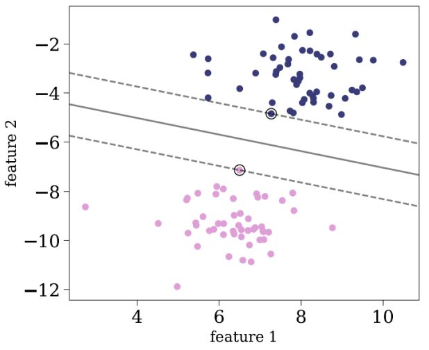Figure 3. Illustration of the SVM best hyperplane for a two-dimensional dataset with linearly-separable classes. The two classes are plotted with pink and purple circles, and the support vectors are marked with black circles. The hyperlane is marked with a solid grey line.

More often than not, the different classes in the dataset are not linearly-separable. The left panel of figure 4 shows an example of a two-dimensional dataset with two classes, which are not linearly-separable (i.e., the classes cannot be separated using a single straight line). The classification problem can be approached with the SVM kernel trick. Instead of constructing the decision boundary in the input data space, the dataset is mapped into a transformed feature space, which is of higher dimension, where linear separation might be possible. Once the decision boundary is found, it is back-projected to the original input space, resulting in a non-linear boundary. The middle panel of figure 4 shows the three-dimensional feature space that resulted from such a mapping, where, in this representation, the classes are linearly-separable. The right panel of figure 4 shows the result of the back-projection of the decision boundary. To apply the kernel trick, one must define the kernel function that is related to the non-linear feature mapping. There is a wide variety of kernel functions, the most popular being Gaussian Radial Basis Function (RBF), Polynomial, and Sigmoid. The kernel function is a hyper-parameter of SVM, and these functions usually depend on additional parameters, which are also hyper-parameters of the model. SVM is available in scikit-learn ⁵.

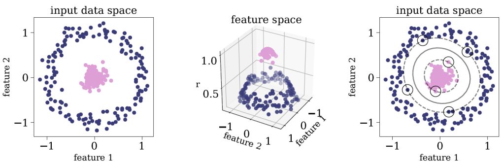Figure 4. Application of the SVM kernel trick to a two-dimensional dataset that consists of two classes which are not linearly-separable. The left panel shows the dataset, where the different classes are represented by pink and purple circles. The middle panel shows the three-dimensional feature space that resulted from the applied mapping, where the classes can be separated with a two-dimensional hyperplane. The right panel shows the result of back-projecting the decision boundary to the input space, where the support vectors are marked with black circles, and the decision boundary with a solid grey line.

2.4. Decision Trees and Random Forest

Ensemble methods are meta-algorithms that combine several supervised learning techniques into a single predictive model, resulting in an overall improved performance, compared to the performance of each individual supervised algorithm. Ensemble methods either combine different supervised learning algorithms, or combine the information of a single algorithm that was trained on different subsets of the training set. One of the most popular ensemble methods is Random Forest, which is a collection of Decision Trees (Breiman et al. 1984; Breiman 2001). Random Forest is mainly used as a supervised algorithm for classification and regression (e.g., Carliles et al. 2010; Bloom et al. 2012; Pichara et al. 2012; Pichara & Protopapas 2013; Möller et al. 2016; Miller et al. 2017; Plewa 2018; Yong et al. 2018; Ishida et al. 2019), but can also be used in an unsupervised setting, to produce similarity measures between the objects in the sample (Shi & Horvath 2006; Baron & Poznanski 2017; Reis et al. 2018a, b).

A decision tree is a non-parametric model constructed during the training stage, which is described by a top-to-bottom tree-like graph, and is used in both classification and regression tasks. The decision tree is a set of consecutive nodes, where each node represents a condition on one feature in the dataset. The conditions are of the form X_j > X_{j, th}, where X_j is the value of the feature at index j and X_{j, th} is some threshold, both of which are determined during the training stage. The lowest nodes in the tree are called terminal nodes or leaves, and they do not represent a condition, but instead carry the assigned label of a particular path within the tree. Figure 5 shows a visualization of a trained decision tree, taken from Vasconcellos et al. (2011), who trained decision tree classifiers to distinguish stars from galaxies.

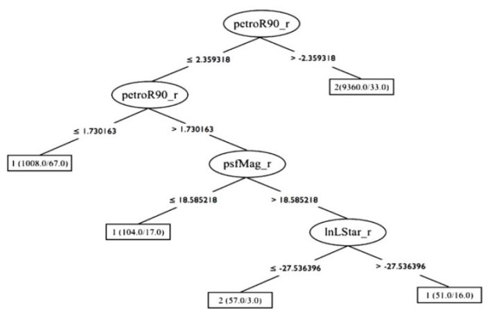Figure 5. An example of a trained decision tree, taken from Vasconcellos et al. (2011). The decision tree contains nodes which represent conditions on features from the dataset, in this case petroR90_r, psfMag_r, and nLStar_r. The terminal nodes represent the assigned label of each particular path within the tree, which are 1, 1, 2, 1, and 2 from left to right, and represent stars and galaxies.

To describe the training process of the decision tree, I consider the simple case of a classification task with two classes. The training process starts with the entire training set in the highest node of the tree – the root. The algorithm searches for the feature X_j and the feature threshold X_{j, th} that result in the best separation of the two classes, where the definition of best separation is a model hyper-parameter, with the typical choices being the Gini impurity or the information gain. Once the best feature and best threshold are determined, the training set propagates to the left and right nodes below the root, according to the established condition. This process is repeated recursively, such that deeper nodes split generally smaller subsets of the original data. In its simplest version, the recursive process stops when every leaf of the tree contains a single class of objects. Once the decision tree is trained, it can be used to predict the class of previously-unseen objects. The prediction is done by propagating the object through the tree, according to its measured features and the conditions in the nodes. The predicted class of the object is then the label of the terminal leaf (for additional information see Breiman et al. 1984; Vasconcellos et al. 2011, Reis et al. 2019).

Decision trees have several advantages. First, in their simpler forms, they have very few hyper-parameters, and can be applied to large datasets with numerous features. Second, their recursive structures are easily interpretable, in particular, they can be used to determine the feature importance. Feature importance represents the relative importance of different features to the classification task at hand. Since the trees are constructed recursively with the aim of splitting the dataset into the predefined classes, features that are selected earlier in the training process, closer to the root, are more important than features that are selected later, closer to the terminal nodes. Obviously, features that were not selected in any node during the training process, carry little relevant information to the classification task. In more complex versions, decision trees can provide a measure of uncertainty for the predicted classes (see e.g., Breiman et al. 1984; Vasconcellos et al. 2011). However, in the simplest version, there are no restrictions on the number of nodes or the depth of the resulting tree, making the algorithm extremely sensitive to outliers. The resulting classifier will typically show a perfect performance on the training set, but a poor performance on new previously-unseen datasets. A single decision tree is typically prone to overfitting the training data, and cannot generalize to new datasets. Therefore, it is rarely used in its single form.

Random Forest is a collection of decision trees, where different decision trees are trained on different randomly-selected subsets of the original training set, and during the training of each individual tree, random subsets of the features are used to construct the conditions in individual nodes. This randomness reduces the correlation between the different trees, resulting in somewhat different tree structures with different conditions in their nodes. The Random Forest prediction is an aggregate of individual predictions of the trees in the forest, in the form of a majority vote. That is, a previously-unseen object is propagated through the different trees, and its assigned label is the label reached in the majority of the trees. While a single decision tree tends to overfit the training data, the combination of many decision trees in the form of a Random Forest generalizes well to previously unseen datasets, resulting in a better performance (for additional information see Breiman 2001). As previously noted, Random Forest is one of the most popular machine learning algorithms in Astronomy.

Random Forest can be applied to datasets with thousands of features, with a moderate increase in running time. The algorithm has a handful of hyper-parameters, such as the number of trees in the forest and the number of randomly-selected features to consider in each node in each tree. In terms of performance, model complexity, and number of hyper-parameters, Random Forest is between SVM and Deep Neural Networks. The main disadvantage of Random Forest, which applies to most supervised learning algorithms, is its inability to take into account feature and label uncertainties. This topic is of particular interest to astronomers, and I discuss it below in section 2.4.1.

Finally, it is worth noting that ensemble methods rely on the construction of a diverse collection of classifiers and aggregation of their predictions (see e.g., Kuncheva & Whitaker 2003). Ensemble methods in the form of "bagging" tend to decrease the classification variance, while methods in the form of "boosting" tend to decrease the classification bias. Random Forest is a "bagging" ensemble method, where the ensemble consists of a diverse collection of individual trees that are trained on different subsets of the data. In "boosting", the decision trees are built sequentially, such that each tree is presented with training samples that the previous tree failed to classify. One of the most popular "boosting" methods in Astronomy is Adaboost (Freund & Schapire 1997). The three algorithms described in this section are available in the scikit-learn library ⁶.

2.4.1. Probabilistic Random Forest

While shown to be very useful for various tasks in Astronomy, many Machine Learning algorithms were not designed for astronomical datasets, which are noisy and have gaps. In particular, measured features typically have a wide range of uncertainty values, and these uncertainties are often not taken into account when training the model. Indeed, the performance of Machine Learning algorithms depends strongly on the signal-to-noise ratio of the objects in the sample, and a model optimized on a dataset with particular noise characteristics will fail on a similar dataset with different noise properties. Furthermore, while in computer vision the labels provided to the algorithm are considered to be "ground truth" (e.g., classification of cats and dogs in images), in Astronomy the labels might suffer from some level of ambiguity. For example, in a classification task of "real" versus "bogus" in transient detection on difference images (see e.g., Bloom et al. 2012), the labels in the training set are obtained from a manual classification of scientists and citizen-scientists. While some might classify a given event as "real", others may classify it as "bogus". In addition, labels in the training set could be the output of a different algorithm, which provides a label with an associated uncertainty. Such uncertainties are also not treated by most Machine Learning algorithms.

Recently, Reis et al. (2019) modified the traditional Random Forest algorithm to take into account uncertainties in the measurements (i.e., features) as well as in the assigned class. The Probabilistic Random Forest algorithm treats the features and the labels as random variables rather than deterministic quantities, where each random variable is represented by a probability distribution function, whose mean is the provided measurement and its variance is the provided uncertainty. Their tests showed that the Probabilistic Random Forest outperforms the traditional Random Forest when applied to datasets with various noise properties, with an improvement of up to 10% in classification accuracy with noisy features, and up to 30% with noisy labels. In addition to the dramatic improvement in classification accuracy, the Probabilistic Random Forest naturally copes with missing values in the data, and outperforms Random Forest when applied to a dataset with different noise characteristics in the training and test sets. The Probabilistic Random Forest was implemented in python and is publicly available on github ⁷.

2.5. Artificial Neural Networks

Artificial neural networks are a set of algorithms with structures that are vaguely inspired by the biological neural networks that constitute the human brain. Their flexible structure and non-linearity allows one to perform a wide variety of tasks, including classification and regression, clustering, and dimensionality reduction, making them extremely popular in Astronomy (e.g., Storrie-Lombardi et al. 1992; Weaver & Torres-Dodgen 1995; Singh et al. 1998; Snider et al. 2001; Firth et al. 2003; Tagliaferri et al. 2003; Vanzella et al. 2004; Blake et al. 2007; Banerji et al. 2010; Eatough et al. 2010; Brescia et al. 2013,, 2014, Ellison et al. 2016; Teimoorinia et al. 2016; Mahabal et al. 2017; Bilicki et al. 2018; Huertas-Company et al. 2018; Naul et al. 2018; Parks et al. 2018; Das & Sanders 2019). In this section I describe the main building blocks of shallow artificial neural networks, and their use for classification and regression tasks. The section does not include details on Deep Learning, in particular Convolutional Neural Networks, Recurrent Neural Networks, and Generative Adversarial Networks (see lectures by M. Huertas-Company for details on deep learning).

Figure 6 is an illustration of a shallow neural network architecture. The network consists of an input layer, output layer, and several hidden layers, where each of these contain neurons that transmit information to the neurons in the succeeding layer. The input data is transmitted from the input layer, through the hidden layers, and reaches the output layer, where the target variable is predicted. The value of every neuron in the network (apart from the neurons in the input layer) is a linear combination of the neurons in the previous layer, followed by an application of a non-linear activation function. That is, the values of the neurons in the first hidden layer are given by ₁ = f₁ (W_{1 0} ), where ₀ is a vector that describes the values of the neurons in the input layer (the input data), W₁ is a weight matrix that describes the linear combination of the input values, and f₁ is a non-linear activation function. In a similar manner, the values of the neurons in the second hidden layer are given by ₂ = f₂ (W_{2 1} ), with a similar notation. Finally, the values of the neurons in the output layer are given by ₃ = f₃ ( W_{3 2} ) = f₃ (W₃ f₂ ( W₂ f₁ ( W_{1 0} ) ) ). The weights of the network are model parameters which are optimized during training via back-propagation (for additional details see lectures by M. Huertas-Company). The non-linear activation functions are model hyper-parameters, with common choices being sigmoid, rectified linear unit function (RELU), hyperbolic tan function (TANH), and softmax. The number of hidden layers and the number of neurons in each of these layers are additional hyper-parameters of the model. The number of neurons in the input and the output layers are defined according to the classification or regression task at hand. Shallow neural networks are available in scikit-learn ⁸.

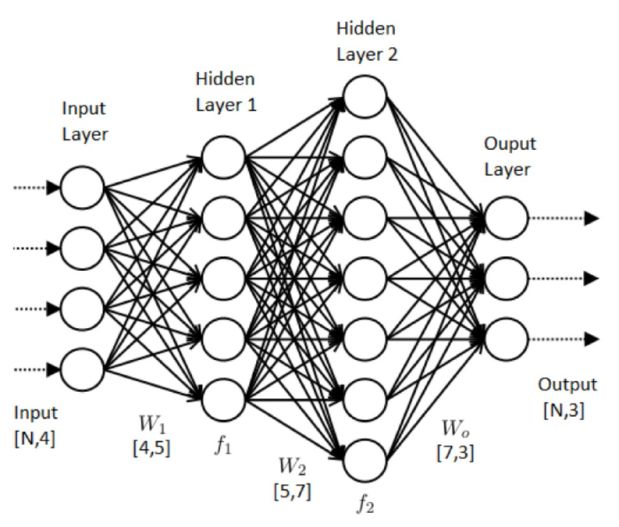Figure 6. Illustration of a shallow neural network architecture. The network consists of an input layer, two hidden layers, and an output layer. The input dataset is propagated from the input layer, through the hidden layers, to the output layer, where a prediction of a target variable is made. Each neuron is a linear combination of the neuron values in the previous layer, followed by an application of a non-linear activation function (see text for more details).

Owing to their flexible structure and non-linearity, artificial neural networks are powerful algorithms, capable of describing extremely complex relations between the input data and the target variable. As just noted, these networks have many hyper-parameters, and they usually require a large amount of data to train on. Furthermore, due to their complexity, they tend to overfit the dataset, and various techniques, such as dropout, are applied to overcome this issue. In addition, these networks are harder to interpret, compared to SVM or Random Forest. However, studies have shown that deep neural networks can greatly outperform traditional algorithms such as SVM, Random Forest, and shallow neural networks, given raw and complex data, such as images, spectra, and light-curves (see e.g., Huertas-Company et al. 2018; Naul et al. 2018; Parks et al. 2018 and references within).

² https://scikit-learn.org/stable/model_selection.html Back.

³ https://scikit-learn.org/stable/modules/feature_selection.html Back.

⁴ https://scikit-learn.org/stable/modules/preprocessing.html Back.

⁵ https://scikit-learn.org/stable/modules/generated/sklearn.svm.SVC.html Back.

⁶ https://scikit-learn.org/stable/modules/generated/sklearn.tree.DecisionTreeClassifier.html
https://scikit-learn.org/stable/modules/generated/sklearn.ensemble.RandomForestClassifier.html
https://scikit-learn.org/stable/modules/generated/sklearn.ensemble.AdaBoostClassifier.html Back.

⁷ https://github.com/ireis/PRF Back.

⁸ https://scikit-learn.org/stable/modules/neural_networks_supervised.html Back.