


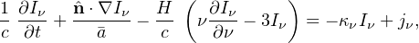
Cosmic reionization can be modeled in a variety of methods, which are depicted in Figure 10. They range from a volume-averaged approach, taking less than a second to compute, to full radiation hydrodynamics cosmological simulations of galaxies and the IGM, taking months to complete. These methods have their advantages and disadvantages, and they complement each other. They use the appropriate observational constraints to make predictions about the reionization history, the nature of its sources, and future observational techniques on further constraining this epoch.
 |
Figure 10. Four different numerical models that capture the process of cosmic reionization: volume-averaged analytic models; spatially-dependent semi-numeric models; radiative transfer calculations that use matter distributions from N-body calculations; full radiation hydrodynamic galaxy formation simulations. The increased physicality and realism comes at the price of added computational cost, limiting the ability to explore different reionization models and the associated parameter space. |
5.1. Volume-averaged analytical models
On the most basic level, reionization models count the number of
ionizing photons and compare it with the number of hydrogen atoms in
some specified volume, which was first (to the best of the
author’s knowledge) studied by Arons & McCray
[93]
in a time-dependent approach. As we have covered in the basic physics of
ionization balance, recombinations can still occur in a strong ionizing
radiation field, and thus cosmic reionization requires more than one
ionizing photon per hydrogen atom. The rate of change in the ionized
fraction xe of the universe can be computed by
considering the comoving photon emissivity
 γ
and recombinations in the ionized regions,
γ
and recombinations in the ionized regions,
 |
(13) |
This differential equation is integrated from a neutral medium (xe = 0) at very early times before any UV sources form (z ∼ 50−100) until the universe is completely ionized (xe = 1). Its evolution gives a reionization history, which then can be integrated to obtain the Thomson scattering optical depth τes.
Here  H is the
mean comoving hydrogen number density,
and
H is the
mean comoving hydrogen number density,
and  rec =
[C αb
H(1 +
Y / 4X)(1 + z)3]−1 is
an effective recombination time. Recall that X = 0.76 and
Y = 1−X are the hydrogen and helium number
fractions, respectively. The clumping factor C ≈
3−5 during EoR accounts for enhanced recombinations in a clumpy
ionized IGM (e.g.
[94,
95]).
There are various definitions for the clumping factor (see
[96] for a discussion),
but the most straightforward definition is C ≡ ⟨
ρ2 ⟩ / ⟨ ρ ⟩2 and
is restricted to ionized regions.
rec =
[C αb
H(1 +
Y / 4X)(1 + z)3]−1 is
an effective recombination time. Recall that X = 0.76 and
Y = 1−X are the hydrogen and helium number
fractions, respectively. The clumping factor C ≈
3−5 during EoR accounts for enhanced recombinations in a clumpy
ionized IGM (e.g.
[94,
95]).
There are various definitions for the clumping factor (see
[96] for a discussion),
but the most straightforward definition is C ≡ ⟨
ρ2 ⟩ / ⟨ ρ ⟩2 and
is restricted to ionized regions.
To calculate the number density of ionizing photons
γ that
escape into the IGM, we first must
calculate the fraction fc of matter that has collapsed
into DM halos and then luminous objects. Most of the uncertainties in
reionization modeling originates from the halo-galaxy connection. More
specifically, given a DM halo, the following main ingredients are needed
to calculate the ionizing emissivity: (i) the star formation rate or
stellar mass, (ii) the stellar ionizing efficiency (i.e. number of
ionizing photons per stellar baryon), and (iii) the UV escape fraction
fesc. For a time and halo mass independent model (e.g.
[97,
98]),
γ =
fesc fγ
 ∗,
where
∗
is the star formation rate density and recall that
fγ is the photon to stellar baryon
ratio. However, simulations have shown that star formation rates and
fesc values are strong functions of halo mass
Mvir. A more accurate value for the ionizing
emissivity can be calculated by integrating over all halo masses,
∗,
where
∗
is the star formation rate density and recall that
fγ is the photon to stellar baryon
ratio. However, simulations have shown that star formation rates and
fesc values are strong functions of halo mass
Mvir. A more accurate value for the ionizing
emissivity can be calculated by integrating over all halo masses,
 |
(14) |
where all of the factors are functions of halo mass, and the
product inside the parentheses is the star formation rate density in
halo masses between M and M + dM. Here
Mmin is the
minimum halo mass that hosts star formation; fgas ≡
Mgas / Mvir is the gas fraction in a
halo; f∗≡ M∗ /
Mgas is the star formation efficiency from
this gas, and
 c is the time
derivative of the
collapsed mass fraction in halos. This integral can be solved
numerically if given functional forms (either smooth or piecewise e.g.
[99,
44]),
which are usually computed from simulations (e.g.
[100])
or semi-analytic models (e.g.
[101])
of early galaxy formation.
c is the time
derivative of the
collapsed mass fraction in halos. This integral can be solved
numerically if given functional forms (either smooth or piecewise e.g.
[99,
44]),
which are usually computed from simulations (e.g.
[100])
or semi-analytic models (e.g.
[101])
of early galaxy formation.
The latest observational constraints strongly suggest that reionization is driven by galaxies and their UV radiation, and thus it is a relatively local process. Semi-numeric models originated from an analytical (excursion set) treatment of reionization [102] that made the fundamental assumption that overdense regions drive reionization. With this assumption, one asserts that if the number of ionizing photons, corrected for recombinations, exceeds the number of baryons in some region, then the region must be ionized. This model has been extended to three-dimensional volumes (e.g. [103, 104, 99]) and can accurately generate full density, velocity, and ionization fields without the need to follow the underlying physics.
From a single set of cosmological initial conditions, usually given in a 3-D lattice with Ncell3 computational cells, at high redshift z ∼ 100, semi-numeric models can compute the ionized fraction for each cell. One major advantage to this method is that these models can calculate xe(r) at any redshift without performing a time-dependent integral. Namely, a cell is considered to be ionized when
 |
(15) |
where ζ is the ionization efficiency, and fc is the collapsed mass fraction inside a sphere of radius R in halos with masses M > Mmin. This value of R is iterated from a large length, usually the UV photon mean free path, down to the width of a single cell. The ionization efficiency can be parameterized (e.g. [56]), not unlike analytical models, to be dependent on the galaxy properties. This method can fully determine the ionization state at any time and position in the volume. The most computationally intensive portion of semi-numeric calculations involves Fast Fourier Transforms (FFTs) and usually takes on the order of core-hours for a single 20483 realization, including the initial condition generation.
5.3. Cosmological radiative transfer simulations
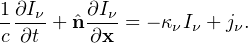
Cosmological N-body simulations evolve the cosmic density field and associated halos, which are then used to calculate the evolution of time- and space-dependent ionization fields. They assume that gas follows the DM, which is a good assumption on large-scales and in larger halos (M ≳ 109 M⊙), and then populate these halos with galaxies that produce ionizing radiation. It is transported through the IGM, usually with ray tracing methods that solve the cosmological radiative transfer equation, which in comoving coordinates [105] is
 |
(16) |
reproducing inhomogeneous reionization. Here
Iν≡ I(ν,
x, Ω, t) is the radiation specific intensity
in units of energy per time t per solid angle per unit area per
frequency ν. H =
 / a is the Hubble
parameter.
/ a is the Hubble
parameter.  = a /
aem
is the ratio of scale factors at the current time and time of
emission. The second term represents the propagation of radiation,
where the factor 1 /
accounts for cosmic
expansion. The third
term describes both the cosmological redshift and dilution of
radiation. On the right hand side, the first term considers the
absorption coefficient κν≡
κν(x, ν, t). The second term
jν≡
jν(x, ν, t) is the emission
coefficient that includes any point sources of radiation or diffuse
radiation.
= a /
aem
is the ratio of scale factors at the current time and time of
emission. The second term represents the propagation of radiation,
where the factor 1 /
accounts for cosmic
expansion. The third
term describes both the cosmological redshift and dilution of
radiation. On the right hand side, the first term considers the
absorption coefficient κν≡
κν(x, ν, t). The second term
jν≡
jν(x, ν, t) is the emission
coefficient that includes any point sources of radiation or diffuse
radiation.
Solving this equation is difficult because of its high dimensionality;
however, we can make some appropriate approximations to reduce its
complexity in order to include radiation transport in numerical
calculations. Typically timesteps in dynamic calculations are small
enough so that Δa / a ≪ 1, therefore
= 1 in any given timestep, reducing the second term to
 ∂
Iν / ∂x. To determine the
importance of the third term, we evaluate the ratio of the third term to
the second term. This is HL / c, where L is the
simulation box length. If this ratio
is ≪ 1, we can ignore the third term. For example at z =
5, this ratio is 0.1 when L = c / H(z = 5) =
53 proper Mpc. In large boxes
where the light crossing time is comparable to the Hubble time, then
it becomes important to consider cosmological redshifting and dilution
of the radiation. Thus equation (16) reduces to the
non-cosmological form in this local approximation,
∂
Iν / ∂x. To determine the
importance of the third term, we evaluate the ratio of the third term to
the second term. This is HL / c, where L is the
simulation box length. If this ratio
is ≪ 1, we can ignore the third term. For example at z =
5, this ratio is 0.1 when L = c / H(z = 5) =
53 proper Mpc. In large boxes
where the light crossing time is comparable to the Hubble time, then
it becomes important to consider cosmological redshifting and dilution
of the radiation. Thus equation (16) reduces to the
non-cosmological form in this local approximation,
 |
(17) |
Ray tracing methods represent the source term jν
as point sources of radiation (e.g. stars, galaxies, quasars) that emit
radial rays that are propagated along the direction
.
The downside to this method is that it neglects any hydrodynamics and must make assumptions about the ionizing luminosity escaping from the halos, the IGM clumping factor C, and the suppression of star formation in low-mass (M ≲ 109 M⊙) halos. Such calculations are performed in either (i) post-processing with the radiative transfer calculated on density field and halo catalog written to disk, or (ii) inline where the halo catalogs and radiation sources are computed on-the-fly, and radiation is traced through the density field that is stored in memory. The largest simulations to-date have over 100 billion particles and simulate domains of over 500 comoving Mpc on a side, and such simulations consume a couple of million core-hours (e.g. [106]). They produce similar results as semi-numeric models but with a larger dynamic range, with higher resolution in collapsed regions, thus can follow the small-scale ionization fluctuations to greater accuracy.
5.4. Full radiation hydrodynamics simulations
Perhaps the most accurate and computationally expensive calculations are full radiation hydrodynamics simulations of cosmological galaxy formation and reionization. Only in the past decade or so, computational resources have become large enough, along with algorithmic advances, to cope with the requirements of such calculations. There are two popular methods to solve the radiative transfer equation coupled to hydrodynamics in three dimensions:
In addition to following the DM dynamics, like in the radiative transfer simulations, they follow the hydrodynamics of the cosmological domain that allows for the treatment of gaseous collapses within halos that are driven by radiative cooling. These radiative processes are computed through a non-equilibrium chemical network (e.g. [120]). However computational run-time and memory limits the resolution of these simulations, which are typically ∼ 10 times more expensive than the cosmological radiative transfer simulations. Depending on the domain size and resolution, ’sub-grid’ star formation prescriptions spawn particles that represent either entire galaxies or individual stellar clusters. Based on this prescription, the particle has an ionizing luminosity, whose radiation is the source of the radiative transfer equation (Equation 16 or 17). Because the radiation transport is coupled with the hydrodynamics, this equation must be solved with either small timesteps and/or the appropriate approximations [116]. Thus, the radiation sources and the ensuing hydrodynamic response can be modeled without relying on a halo-galaxy relationship. The suppression of star formation, especially in low-mass galaxies can be directly modeled, along with the regulation of star formation that results in a more accurate description of the ionizing sources during the EoR and the process of reionization itself. That being said, there still exists uncertainties, arising from the sub-grid models and convergence issues of the numerical solvers with respect to resolution.