

6.2 A basic observational diagram
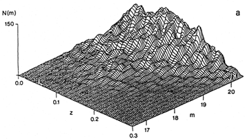
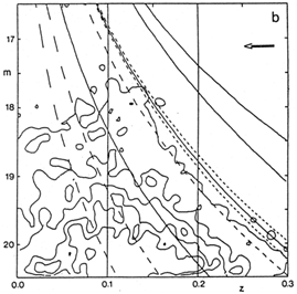
Measurements are made of magnitudes and redshifts; the number of galaxies per magnitude and redshift interval is counted. The three-dimensional version of the diagram is shown in Fig. 31a. The bias towards certain redshift-magnitude combinations is clearly visible. A two-dimensional projection is shown in Fig. 31b. Various computed curves are inserted in the diagram; their parameters are given in Table 1.

|

|
Figure 31. Basic observational diagram:
m, z, N (m, z)
(Seitter et
al. 1988).
The two vertical lines are the projections of curves following the N (m)-'landscape'. They correspond to observational luminosity functions before normalization. H0 is given in km s-1 Mpc-1. |
| Curve | H0 | q0 | 
| M | K |
| solid solid | 100 100 | 0.5 0.5 | 0 0 | -22 -22 | 2.0 z 4.0 z |
| solid solid | 100 50 | 0.5 0.5 | 0 0 | -21 -21 | 4.14 z - 0.44 z2 4.14 z - 0.44 z2 |
| dotted dotted | 100 100 | 0.1 1.0 | 0 0 | -21 -21 | 4.14 z - 0.44 z2 4.14 z - 0.44 z2 |
| dashed dashed dashed | 75 75 75 | 0.5 0.5 0.5 | 0 0 0 | -21.5 -19.5 -18.5 | 4.14 z - 0.44 z2 4.14 z - 0.44 z2 4.14 z - 0.44 z2 |