2. FIRST-ORDER DIFFERENCE EQUATIONS

One of the simplest systems an ecologist can study is a seasonally breeding population in which generations do not overlap ^{1 - 4}. Many natural populations, particularly among temperate zone insects (including many economically important crop and orchard pests), are of this kind, In this situation, the observational data will usually consist of information about the maximum, or the average, or the total population in each generation. The theoretician seeks to understand how the magnitude of the population in generation t+1, X_t+1, is related to the magnitude of the population in the preceding generation t, X_t: such a relationship may be expressed in the general form

The function F(X) will usually be what a biologist calls "density dependent", and a mathematician calls nonlinear; equation (1) is then a first-order, nonlinear difference equation.

Although I shall henceforth adopt the habit of referring to the variable X as "the population", there are countless situations outside population biology where the basic equation (1), applies. There are other examples in biology, as, for example in genetics ^{5, 6} (where the equation describes the change in gene frequency in time) or in epidemiology ⁷ (with X the fraction of the population infected at time t). Examples in economics include models for the relationship between commodity quantity and price ⁸, for the theory of business cycles ⁹, and for the temporal sequences generated by various other economic quantities ¹⁰. The general equation (1) also is germane to the social sciences ¹¹, where it arises, for example, in theories of learning (where X may be the number of bits of information that can be remembered after an interval t), or in the propagation of rumours in variously structured societies (where X is the number of people to have heard the rumour after time t). The imaginative reader will be able to invent other contexts for equation (1).

In many of these contexts, and for biological populations in particular, there is a tendency for the variable X to increase from one generation to the next when it is small, and for it to decrease when it is large. That is, the nonlinear function F(X) often has the following properties: F(0)=0; F(X) increases monotonically as X increases through the range 0 < X < A (with F(X) attaining its maximum value at X = A); and F(X) decreases monotonically as X increases beyond X = A. Moreover, F(X) will usually contain one or more parameters which "tune" the severity of this nonlinear behaviour; parameters which tune the steepness of the hump in the F(X) curve. These parameters will typically have some biological or economic or sociological significance.

A specific example is afforded by the equation ^{1, 4, 12 - 23}

This is sometimes called the "logistic" difference equation. In the limit b = 0, it describes a population growing purely exponentially (for a > 1); for b 0, the quadratic nonlinearity produces a growth curve with a hump, the steepness of which is tuned by the parameter a. By writing X = bN/a, the equation may be brought into canonical form ^{1, 4, 12 - 23}

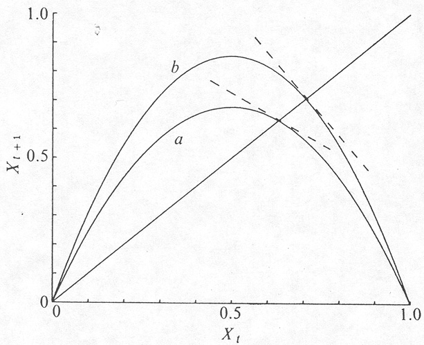
In this form, which is illustrated in Fig. 1, it is arguably the simplest nonlinear difference equation. I shall use equation (3) for most of the numerical examples and illustrations in this article. Although attractive to mathematicians by virtue of its extreme simplicity, in practical applications equation (3) has the disadvantage that it requires X to remain on the interval 0 < X < 1; if X ever exceeds unity, subsequent iterations diverge towards - (which means the population becomes extinct). Furthermore, F(X) in equation (3) attains a maximum value of a/4 (at X = 1/2); the equation therefore possesses non-trivial dynamical behaviour only if a < 4. On the other hand, all trajectories are attracted to X = 0 if a < 1. Thus for non-trivial dynamical behaviour we require 1 < a < 4; failing this, the population becomes extinct.

Figure 1. A typical form for the relationship between Xt+1 and Xt described by equation (1). The curves are for equation (3), with a = 2.707 (a); and a = 3.414 (b). The dashed lines indicate the slope at the "fixed points" where F(X) intersects the 45° line: for the case a this slope is less steep than -45° and the fixed point is stable; for b the slope is steeper than -45°, and the point is unstable.

Another example, with a more secure provenance in the biological literature 1, 23 - 27, is the equation

This again describes a population with a propensity to simple exponential growth at low densities, and a tendency to decrease at high densities. The steepness of this nonlinear behaviour is tuned by the parameter r. The model is plausible for a single species population which is regulated by an epidemic disease at high density ²⁸. The function F(X) of equation (4) is slightly more complicated than that of equation (3), but has the compensating advantage that local stability implies global stability¹ for all X > 0.

The forms (3) and (4) by no means exhaust the list of single-humped functions F(X) for equation (1) which can be culled from the ecological literature. A fairly full such catalogue is given, complete with references, by May and Oster ¹. Other similar mathematical functions are given by Metropolis et al. ¹⁶. Yet other forms for F(X) are discussed under the heading of "mathematical curiosities" below.