3. DYNAMIC PROPERTIES OF EQUATION (1)

Possible constant, equilibrium values (or "fixed points") of X in equation (1) may be found algebraically by putting X_t+1 = X_t = X*, and solving the resulting equation

An equivalent graphical method is to find the points where the curve F(X) that maps X_t into X_t+1 intersects the 45° line, X_t+1 = X_t which corresponds to the ideal nirvana of zero population growth; see Fig. 1. For the single-hump curves discussed above, and exemplified by equations (3) and (4), there are two such points: the trivial solution X = 0, and a non-trivial solution X* (which for equation (3) is X* = 1 - (1/a).

The next question concerns the stability of the equilibrium point X*. This can be seen ^{24, 25, 19 - 21, 1, 4} to depend on the slope of the F(X) curve at X*. This slope, which is illustrated by the dashed lines in Fig. 1, can be designated

(X*) = [dF / dX]_{x = x*}         (6)

So long as this slope lies between 45° and -45° (that is, ⁽¹⁾ between +1 and -1), making an acute angle with the 45° ZPG line, the equilibrium point X* will be at least locally stable, attracting all trajectories in its neighbourhood. In equation (3), for example, this slope is ⁽¹⁾ = 2 - a: the equilibrium point is therefore stable, and attracts all trajectories originating in the interval 0 < X < 1, if and only if 1 < a < 3.

As the relevant parameters are tuned so that the curve F(X) becomes more and more steeply humped, this stability-determining slope at X* may eventually steepen beyond -45° (that is, ⁽¹⁾ < -1), whereupon the equilibrium point X* is no longer stable.

What happens next? What happens, for example, for a > 3 in equation (3)?

To answer this question, it is helpful to look at the map which relates the populations at successive intervals 2 generations apart; that is, to look at the function which relates X_t+2 to X_t. This second iterate of equation (1) can be written

or, introducing an obvious piece of notation,

The map so derived from equation (3) is illustrated in Figs 2 and 3.

Figure 2. The map relating Xt+2 to Xt, obtained by two iterations of equation (3). This figure is for the case (a) of Fig. 1, a = 2.707: the basic fixed point is stable, and it is the only point at which F(2)(X) intersects the 45° line (where its slope, shown by the dashed line, is less steep than 45°).

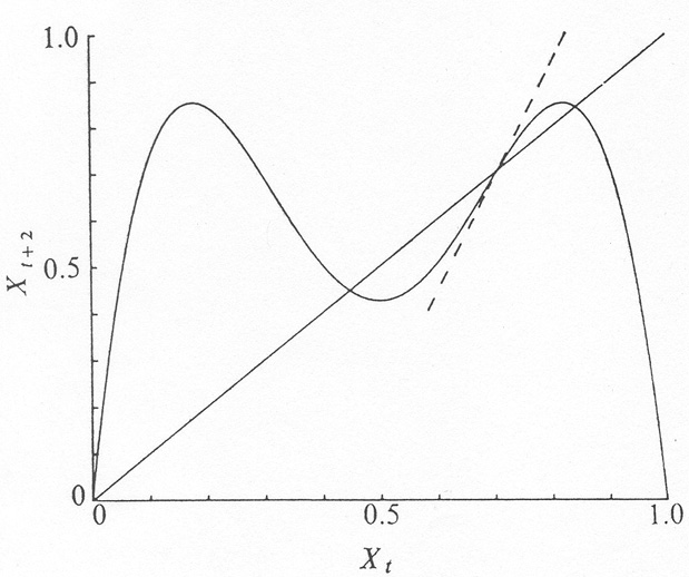
Figure 3. As for Fig. 2, except that here a = 3.414, as in Fig. 1b. The basic fixed point is now unstable: the slope of F(2)(X) at this point steepens beyond 45°, leading to the appearance of two new solutions of period 2.

or graphically from the intersection between the map F⁽²⁾(X) and the 45° line, as shown in Figs 2 and 3. Clearly the equilibrium point X* of equation (5) is a solution of equation (9); the basic fixed point of period 1 is a degenerate case of a period 2 solution. We now make a simple, but crucial, observation ¹: the slope of the curve F⁽²⁾(X) at the point X*, defined as ⁽²⁾(X*) and illustrated by the dashed lines in Figs 2 and 3, is the square of the corresponding slope of F(X)

⁽²⁾ (X*) = [⁽¹⁾ (X*)]²         (10)

This fact can now be used to make plain what happens when the fixed point X* becomes unstable. If the slope of F(X) is less than -45° (that is, |⁽¹⁾| < 1), as illustrated by curve a in Fig. 1, then X* is stable. Also, from equation (10), this implies 0 < ⁽²⁾ < 1 corresponding to the slope of F⁽²⁾ at X* lying between 0° and 45°, as shown in Fig. 2. As long as the fixed point X* is stable, it provides the only non-trivial solution to equation (9). On the other hand, when ⁽¹⁾ steepens beyond -45° (that is, |⁽¹⁾| > 1), as illustrated by curve b in Fig 1, X* becomes unstable. At the same time, from equation (10) this implies ⁽²⁾ > 1, corresponding to the slope of F⁽²⁾ at X* steepening beyond 45°, as shown in Fig. 3. As this happens, the curve F⁽²⁾(X) must develop a "loop", and two new fixed points of period 2 appear, as illustrated in Fig. 3.

In short, as the nonlinear function F(X) in equation (1) becomes more steeply humped, the basic fixed point X* may become unstable. At exactly the stage when this occurs, there are born two new and initially stable fixed points of period 2, between which the system alternates in a stable cycle of period 2. The sort of graphical analysis indicated by Figs 1, 2 and 3, along with the equation (10), is all that is needed to establish this generic result ^{1, 4}.

As before, the stability of this period 2 cycle depends on the slope of the curve F⁽²⁾(X) at the 2 points. (This slope is easily shown to be the same at both points ^{1, 20}, and more generally to be the same at all k points on a period k cycle.) Furthermore, as is clear by imagining the intermediate stages between Figs 2 and 3, this stability-determining slope has the value = +1 at the birth of the 2-point cycle, and then decreases through zero towards = -1 as the hump in F(X) continues to steepen. Beyond this point the period 2 points will in turn become unstable, and bifurcate to give an initially stable cycle of period 4. This in turn gives way to a cycle of period 8, and thence to a hierarchy of bifurcating stable cycles of periods 16, 32, 64,..., 2ⁿ. In each case, the way in which a stable cycle of period k becomes unstable, simultaneously bifurcating to produce a new and initially stable cycle of period 2k, is basically similar to the process just adumbrated for k = 1. A more full and rigorous account of the material covered so far is in ref. 1.

This "very beautiful bifurcation phenomenon" ²² is depicted in Fig. 4, for the example equation (3). It cannot be too strongly emphasised that the process is generic to most functions F(X) with a hump of tunable steepness. Metropolis et al. ¹⁶ refer to this hierarchy of cycles of periods 2ⁿ as the harmonics of the fixed point X*.

Figure 4. This figure illustrates some of the stable ( ___ ) and unstable (----) fixed points of various periods that can arise by bifurcation processes in equation (1) in general, and equation (3) in particular. To the left, the basic stable fixed point becomes unstable and gives rise by a succession of pitchfork bifurcations to stable harmonics of period 2n; none of these cycles is stable beyond a = 3.5700. To the right, the two period 3 cycles appear by tangent bifurcation: one is initially unstable; the other is initially stable, but becomes unstable and gives way to stable harmonics of period 3 × 2n, which have a point of accumulation at a = 3.8495. Note the change in scale on the a axis, needed to put both examples on the same figure. There are infinitely many other such windows, based on cycles of higher periods.

Beyond this point of accumulation (for example, for a > a_c in equation (3)) there are an infinite number of fixed points with different periodicities, and an infinite number of different periodic cycles. There are also an uncountable number of initial points X₀ which give totally aperiodic (although bounded) trajectories; no matter how long the time series generated by F(X) is run out, the pattern never repeats. These facts may be established by a variety of methods 1, 4, 20, 22, 29. Such a situation, where an infinite number of different orbits can occur, has been christened "chaotic" by Li and Yorke²⁰.

As the parameter increases beyond the critical value, at first all these cycles have even periods, with X_t alternating up and down between values above, and values below, the fixed point X*. Although these cycles may in fact be very complicated (having a non-degenerate period of, say, 5,726 points before repeating), they will seem to the casual observer to be rather like a somewhat "noisy" cycle of period 2. As the parameter value continues to increase, there comes a stage (at a = 3.6786.. for equation (3)) at which the first odd period cycle appears. At first these odd cycles have very long periods, but as the parameter value continues to increase cycles with smaller and smaller odd periods are picked up, until at last the three-point cycle appears (at a = 3.8284 . . for equation (3)). Beyond this point, there are cycles with every integer period, as well as an uncountable number of asymptotically aperiodic trajectories: Li and Yorke ²⁰ entitle their original proof of this result "Period Three Implies Chaos".

The term "chaos" evokes an image of dynamical trajectories which are indistinguishable from some stochastic process. Numerical simulations ^{12, 15, 21, 23, 25} of the dynamics of equation (3), (4) and other similar equations tend to confirm this impression. But, for smooth and "sensible" functions F(X) such as in equations (3) and (4), the underlying mathematical fact is that for any specified parameter value there is one unique cycle that is stable, and that attracts essentially all initial points ^{22, 29} (see ref. 4, appendix A, for a simple and lucid exposition). That is, there is one cycle that "owns" almost all initial points; the remaining infinite number of other cycles, along with the asymptotically aperiodic trajectories, own a set of points which, although uncountable, have measure zero.

As is made clear by Tables 3 and 4 below, any one particular stable cycle is likely to occupy an extraordinarily narrow window of parameter values. This fact, coupled with the long time it is likely to take for transients associated with the initial conditions to damp out, means that in practice the unique cycle is unlikely to be unmasked, and that a stochastic description of the dynamics is likely to be appropriate, in spite of the underlying deterministic structure. This point is pursued further under the heading "practical applications", below.

The main messages of this section are summarised in Table 1, which sets out the various domains of dynamical behaviour of the equations (3) and (4) as functions of the parameters, a and r respectively, that determine the severity of the nonlinear response. These properties can be understood qualitatively in a graphical way, and are generic to any well behaved F(X) in equation (1).

Table 1. Summary of the way various "single-hump" functions F(X), from equation (1), behave in the chaotic region, distinguishing the dynamical properties which are generic from those which are not

The function F(X)			aX; if X < ½	X; if X < 1
of equation (1)	aX(1 - X)	X exp[r(1 - X)]	a(1 - X); if X > ½	X1-b; if X > 1
Tunable parameter	a	r	a	b
Fixed point becomes unstable	3.0000	2.0000	1.0000*	2.0000
"Chaotic" region begins
[point of accumulation of cycles of period 2n]	3.5700	2.6924	1.0000	2.0000
First odd-period cycle appears	3.6786	2.8332	1.4142	2.6180
Cycle with period 3 appears
[and therefore every integer period present]	3.8284	3.1024	1.6180	3.0000
"Chaotic" region ends	4.0000†	‡	2.000†	‡
Are there stable cycles in the chaotic region?	Yes	Yes	No	No
* Below this a value, X = 0 is stable.
† All solutions are attracted to - for a values beyond this.
‡ In practice, as r or b becomes large enough, X will eventually be carried so low as to be effectively zero, thus producing extinction in models of biological populations.

We now proceed to a more detailed discussion of the mathematical structure of the chaotic regime for analytical functions, and then to the practical problems alluded to above and to a consideration of the behavioural peculiarities exhibited by non-analytical functions (such as those in the two right hand columns of Table 1).