


3.5. Transfer Function Recovery
With data of sufficient quality, transfer functions for different plausible models are distinguishable from one another. This is of course, why we place so much emphasis on them: if we can determine the transfer function for a particular line, we have very strong constraints on the geometry and kinematics of the responding region, and if the BLR has a spherically or azimuthally symmetric structure, it may be possible to determine the BLR kinematics and structure with fairly high accuracy and strongly constrain the emission-line reprocessing physics. The operational goal of reverberation mapping experiments is thus to determine the transfer functions for various emission lines in AGN spectra.
How can we determine the transfer functions from observational data? Inspection of the transfer equation (Eq. (20)) immediately suggests Fourier inversion (i.e., the method of Fourier quotients), which was the formulation outlined by Blandford & McKee 7 . We define the Fourier transform of the continuum light curve C(t) as
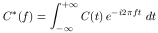
| (28) |
and similarly define the Fourier transform of the line light curve. By the convolution theorem 9, the transfer function becomes

| (29) |
so that  * = L* / C*, and
the transfer function is obtained from
* = L* / C*, and
the transfer function is obtained from
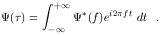
| (30) |
In practice, however, Fourier methods are not used as they are inadequate when applied to data that are relatively noisy (i.e., flux uncertainties are only a factor of a few to several smaller than the variations) and which are limited in terms of both sampling rate, which is in any case usually irregular, and duration. Simpler methods, like cross-correlation (Sec. 4), can be applied with success, though with limited results. Cross-correlation, we will see, can give the first moment of the transfer function, but little else.
In principle, more powerful methods can be used to attempt to recover transfer functions. The most commonly used is the Maximum Entropy Method (MEM) 33. MEM is a generalized version of maximum likelihood methods, such as least-squares. The difference is that in the method of least squares, a parameterized model is fitted to the data, whereas MEM finds the "simplest" (maximum entropy) solution, balancing model simplicity and realism. Examples of MEM solutions will be shown in Sec. 5. Other methodologies that have been employed for transfer-function solution include subtractively optimized local averages (SOLA) 77 and regularized linear inversion 44.