© CAMBRIDGE UNIVERSITY PRESS 2000

13.2. Epicyclic orbits

In the limit of quasi-circular orbits, which can be quantified as

(13.17)

we have _r(E, J) (r₀), (E, J) (r₀) and the radial periodic motion can be approximated by a harmonic oscillator with the epicyclic frequency defined by:

(13.18)

(We also have J_r ~ [E - E₀(r₀)] / (r₀), which is analogous to v² / B for a gyrating charged particle in a magnetic field.) Thus if we separate out the motion of the guiding center by writing r(t) = r₀ + r₁(t) and (t) = (r₀) + ₁(t), the linearized equation for the conservation of angular momentum leads to:

(13.19)

thus the epicycles are ellipses characterized by aspect ratio 2 / (therefore they are usually elongated in the direction of the motion), with the star running in the opposite direction with respect to the guiding center (i.e., the motion in the epicycle is clockwise if the motion on the circular orbit at r₀ is counter-clockwise).

Note that from Eq. (18) the condition for the stability of circular orbits (² > 0) formally coincides with the classical Rayleigh's criterion for the stability of a rotating fluid ⁽⁴⁾. A few important special cases should be noted. A pure harmonic potential (i.e., the mean field potential associated with a homogeneous sphere) implies solid body rotation, in the sense that ² = 4 G /3 = constant; in this case we have = 2, and orbits are closed in the form of ellipses centered at r = 0. A point mass generates a Keplerian potential; from the third law of planetary motion we see that in this case = , and thus orbits are closed in the form of ellipses with one focus at r = 0. For galaxy disks, since they are often characterized by a flat rotation curve, the typical relation should be 2^1/2 , and orbits are generally not closed. Some simple cases of orbits with and in rational ratio are shown in Fig. 13.3.

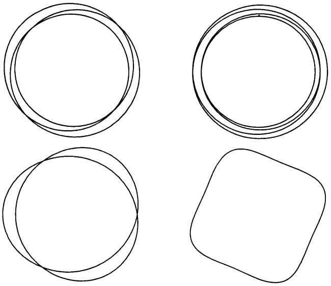Figure 13.3. Quasi-circular orbits when the ratio of angular to radial frequency is rational (3/2, upper left; 2/3 lower left; 4, upper right; 1/4, lower right). (In a frame rotating with angular velocity p the relevant angular frequency is the frequency in the inertial frame reduced by the value of p)

For some purposes (e.g. for some detailed stellar dynamical studies of density waves where an integration along the unperturbed orbits is performed), it is of interest to have a full description of the epicyclic expansion, beyond the lowest order harmonic oscillator obtained by approximating the potential _eff with a parabola in r₀. Such a systematic expansion ⁽⁵⁾ is obtained by introducing an appropriate phase variable . In order to do this, it is first convenient to consider the transformation (E, J) (a, r₀), where the dimensionless epicyclic energy a is given by

(13.20)

Thus the radial momentum can be expressed as a function

(13.21)

Now the phase variable is introduced by replacing the radial velocity coordinate p_r with

(13.22)

The complete epicyclic expansion is thus obtained by Taylor expansion of Eq. (21) around r = r₀, which inserted in Eq. (22) gives

(13.23)

From here one gets the expression for dr / d as well. Then from

(13.24)

(13.25)

one gets the desired expressions for = (t) and = (t), which completes the derivation. The first terms of the full expansion can be summarized by noting

(13.26)

(13.27)

with B₃ = - A₃ + 2A₂ - 1 and

(13.28)

Here one can easily check that for the harmonic oscillator A₂ = 1/2 and A₃ = B₃ = 0, while for the Keplerian case A₂ = 0, A₃ = 0, B₃ = -1. Note that for the isochrone potential (see Chapter 21) A₁ = 1 and all the other A_n vanish.

Many of these results find application in the study of the dynamics of galaxies. In addition, they are also of interest in some simple problems of celestial mechanics, where the potential is often close to being Keplerian. For example, the potential of the Earth, in space (r > r_T), because of its flattening at the poles, is approximately given by

(13.29)

where we have retained only the quadrupole term in the general solution to the Laplace equation (here at r = r_T the quantity /2 - represents the geographical latitude); for the Earth one has J₂₀ 10^-3. We recall the expression for the Legendre polynomial P₂₀(x) = (3x2 - 1)/2. The epicyclic theory easily allows us to study the precession of the perigee of a satellite on the equatorial plane, where = /2. The precession rate is proportional to the difference between and .

⁴ See, for example, Chandrasekhar, S. (1961), Hydrodynamic and Hydromagnetic Stability, Oxford University Press, Oxford; reprinted by Dover Back.

⁵ Shu, F.H. (1969), Astrophys. J., 158, 505; Mark, J.W-K. (1976), Astrophys. J., 203, 81. The analysis of Mark removes an undesired secular term present in the original derivation Back.