


The turnover in the radio spectrum is a defining characteristic of the GPS and CSS sources. It contains information on the source size, its physical properties, and its environment.
2.1. Spectral Shape and Implications for Lifetimes
The shapes of the radio spectra are one of the chief identifying
characteristics of the GPS and CSS sources (see
Fig. 1 and
Fanti et al. 1985,
1989;
Schilizzi et al. 1990;
Steppe, Salter, &
Saikia 1990;
O'Dea et al. 1990b;
Kameno et al. 1995;
Steppe et al. 1995;
Stanghellini et al. 1996,
1998b;
de Vries et al. 1997a).
These sources have simple peaked spectra with steep spectral indices at
high frequencies. O'Dea et al.
(1990b,
1991)
noted that the spectra of GPS sources can be quite narrow with values
for the full width to half the peak flux density of around 1-1.5 decades
of frequency. The GPS source with the most inverted spectrum is 0108+388
(Baum et al. 1990),
which has a value of 
 2 and approaches
the canonical value of 2.5 for a simple homogeneous synchrotron
source. However, the fact that none of the GPS or CSS sources have
spectra as inverted as 2.5 suggests that there is inhomogeneity in the
radio structure (this is of course confirmed by the radio imaging
[section 3], which shows cores, jets, hot
spots, and lobes in these objects).
2 and approaches
the canonical value of 2.5 for a simple homogeneous synchrotron
source. However, the fact that none of the GPS or CSS sources have
spectra as inverted as 2.5 suggests that there is inhomogeneity in the
radio structure (this is of course confirmed by the radio imaging
[section 3], which shows cores, jets, hot
spots, and lobes in these objects).
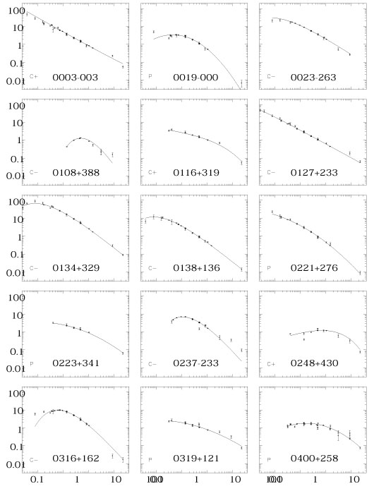 |
Figure 1. Radio spectra of GPS and CSS radio sources (S. Jeyakumar 1997, private communication; see also Steppe et al. 1995). Vertical axis is flux density in Jy, and horizontal axis is frequency in GHz. |
The distribution of spectral index above the peak is shown in
Figure 2. This plot combines the data for the
Fanti et al. (1990b)
sample of CSSs and the
Stanghellini et
al. (1998b)
sample of GPSs (shaded). The lower limit at about -0.5 is imposed
by the selection criteria. (3)
There is a broad distribution from -0.5 to -1 with a few sources around
-1.1 to -1.3. (4) The GPS and
CSS sources have similar distributions. There is a slight suggestion
that the GPS sources have flatter spectra than the CSSs, but this may be
mainly a result of the fact that the spectral indices are measured
closer to the spectral peak in the GPSs than in the CSSs.
de Vries et al. (1997a)
have determined an "average" radio spectrum for a sample of 72 GPS radio
sources. The average spectral indices below and above the spectral peak
are 0.56 and -0.77, respectively. The average value of
 -0.77 is also typical
for the large-scale powerful sources (see, e.g.,
Kellermann 1966b),
suggesting that relativistic electron acceleration and energy loss
mechanisms preserve the same average spectral index over most of the
lifetime of the source.
-0.77 is also typical
for the large-scale powerful sources (see, e.g.,
Kellermann 1966b),
suggesting that relativistic electron acceleration and energy loss
mechanisms preserve the same average spectral index over most of the
lifetime of the source.
 |
Figure 2. Histogram of spectral index above the spectral peak. The sources are the Fanti et al. CSS sample and the Stanghellini et al. GPS sample (shaded). |
If the turnover is due to synchrotron self-absorption, then from equation (2) the generally narrow spectrum implies that there is a limited range of spatial scales that contribute to the bulk of the radio luminosity; i.e., there is a cutoff in both the largest and smallest scales (see also Phinney 1985). This is consistent with the lack of large-scale structure in these sources.
The spectra tend to be fairly straight (constant spectral index) at high
frequencies with few sources showing either steepening from radiation
losses, or flattening due to a compact component (though there are
examples of both phenomena). This has consequences for the inferred
"spectral age" of the radiating electrons. Two possible explanations for
the lack of an observed break are that the spectral break is either (1)
still at higher frequencies
(100 GHz) or (2)
hidden below the spectral peak. As pointed out by
Kardashev (1962),
continuous resupply will limit the change in spectral index at the break
frequency to 0.5 instead of an exponential drop. Thus, if the jets
supply sufficient energy to the extended radio structure that
Kardashev's condition is met, it is possible that the break is below the
spectral peak for the sources with a high-frequency spectral index
steeper than -1. For sources with flatter spectra the implied initial
spectrum
-0.5 may be too
flat to be consistent with the extended optically thin emission, and
these sources may have their break at high frequency. Because of both
continuing resupply and adiabatic losses, which will have opposite
effects on the spectrum, the interpretation of the spectral age is
uncertain. The electron lifetime is given by
 |
(1) |
where B is the magnetic field in G, BR
4(1 +
z)2 × 10⁻⁶ G is the equivalent magnetic
field of the microwave background, and
 b is the
break frequency in Hz
(van der Laan &
Perola 1969).
For a high value of break frequency
b = 100 GHz,
for a GPS source (B = 10-3 G) and a CSS source
(B = 10-4 G), the electron lifetimes are t
2 × 10³
yr and t
7 × 10⁴
yr, respectively. However, for a low value of the break frequency
b = 100 MHz,
the ages are t
7 × 10⁴
yr and t
2 × 10⁶
yr, respectively. Given the uncertainties, the range of spectral indices
is consistent with a range of electron lifetimes among these sources,
with some sources having possibly quite short electron lifetimes. The
correspondence between electron lifetime and source age is not yet clear
- though these results could be consistent with a range of ages for the
GPS and CSS sources, with some of them, especially the GPS sources with
flatter spectra, being quite young
(
b is the
break frequency in Hz
(van der Laan &
Perola 1969).
For a high value of break frequency
b = 100 GHz,
for a GPS source (B = 10-3 G) and a CSS source
(B = 10-4 G), the electron lifetimes are t
2 × 10³
yr and t
7 × 10⁴
yr, respectively. However, for a low value of the break frequency
b = 100 MHz,
the ages are t
7 × 10⁴
yr and t
2 × 10⁶
yr, respectively. Given the uncertainties, the range of spectral indices
is consistent with a range of electron lifetimes among these sources,
with some sources having possibly quite short electron lifetimes. The
correspondence between electron lifetime and source age is not yet clear
- though these results could be consistent with a range of ages for the
GPS and CSS sources, with some of them, especially the GPS sources with
flatter spectra, being quite young
( 104
yr).
Katz-Stone & Rudnick
(1997)
have presented a "spectral tomography" analysis of two CSS sources,
3C 67 and 3C 190. They find complex spectral structure in
these two sources
and suggest that the sources could be young if the initial injection
spectrum is as steep as
-0.8. It is clear that
images of spectral index are necessary to fully address the questions of
electron age and source lifetime.
104
yr).
Katz-Stone & Rudnick
(1997)
have presented a "spectral tomography" analysis of two CSS sources,
3C 67 and 3C 190. They find complex spectral structure in
these two sources
and suggest that the sources could be young if the initial injection
spectrum is as steep as
-0.8. It is clear that
images of spectral index are necessary to fully address the questions of
electron age and source lifetime.
3 Note that there is some small inconsistency, since the updated values of spectral index used here are not the same as those originally used to define these samples. Back.
4 Curiously, the spectra can be as steep as those of the high-redshift ultrasteep-spectrum sources (see, e.g., Röttgering et al. 1994).