© CAMBRIDGE UNIVERSITY PRESS 1999

7. The Expanding Search for Homogeneity

Over all scales on which astronomers had looked, from planets to clusters of galaxies, the distribution was nonuniform. Yet, the intuition of great observers like Hubble suggested there would be a scale without structure. Where was it?

Perhaps it was nowhere; perhaps it was everywhere. Every scale might be clustered, but in the same manner, so there was no distinction between scales. This self-similar picture is more subtle than the idea that the Universe suddenly becomes uniform at a particular very large scale. Carpenter (1938) suggested that it followed from his earlier (Carpenter, 1931) discovery of a single relation between the number of galaxies in a cluster and the cluster radius. He refined this relation in 1938 to the form N R_c^1.5. Although he considered this to be an upper bound of the N - R_c distribution, it also provides a good fit through his data. Since it applied over three orders of magnitude in N, he concluded in the later paper "that there is no essential distinction between the large, rich clusters and the smaller groups, the total populations and other characteristics varying gradually from one extreme to the other."

Without realizing it, Carpenter had found the first evidence for the form of the two-point correlation function (r) and, indirectly, for the fractal nature of the galaxy distribution. From Equation (6.8), the excess number of galaxies (above the average number in a Poisson distribution) around a galaxy is N_c = 4 r² (r) dr. Over small scales where >> 1 we expect N_c N, the number of galaxies in the cluster. Therefore if (r) is a power law, as Carpenter might have expected in his self-similar picture, then N_c r^1.5 implies r^-1.5.

This is not far from the typical modem value r^-1.8. Furthermore, if the number density of galaxies were uniform, we would expect N r³. In a more general fractal distribution N ~ r^3-d. (see Chapter 12): 50 Carpenter essentially found the fractal dimension d = 1.5. Actually the situation is not quite so simple because the form of (r) and the fractal dimension both turn out to depend upon scale (see Chapters 12, 14, and 20).

Zwicky (1937, 1938) came to a similar conclusion that nearly all galaxies were clustered on all scales, rather than most galaxies being part of a fairly uniform field distribution with a sprinkling of dense clusters. He also described the concentration of elliptical galaxies in clusters, suggesting this was caused by mass segregation. And he attempted to calculate the spatial distribution function of galaxies, assuming a Boltzmann energy distribution and no statistical evolution of the system of galaxies. Although this missed the essential gravitational physics of the problem, like the attempts of Lemaitre and Milne, and although Zwicky's program could not be calculated, it helped open a significant question: Could statistical mechanics describe the galaxy distribution?

Thus by the late 1950s there was a consensus that galaxies did not have a Poisson distribution, even though the description of their clustering was unclear. Disputes centered over whether the essential feature was self-similar hierarchical clustering, or a few large clusters in a uniform field, or the specific distributions of cluster forms and separations that Neyman and Scott proposed, or fits to ad hoc forms of the two-point correlation function. Relations among some of these descriptions were beginning to emerge along with a rudimentary understanding of their underlying physics.

At this stage, the scale expanded. Why not repeat the galaxy clustering analyses with the clusters themselves, considering each cluster as a point mass? Are the clusters clustered? And so the great superclustering controversy began.

It was abetted by the construction of two different cluster catalogs, each defining clusters differently and subject to different selection effects. The discussion almost mimicked the earlier controversy between Hubble and Shapley, with their two different galaxy catalogs. Previously the discovery of clusters, like the earliest discoveries of galaxies, had been a rather haphazard affair. As usual, the most prominent and often least representative ones were noticed firstl To systematize this process, Abell (1958) examined 879 pairs of photographs in the National Geographic Society-Palomar Observatory Sky Survey made with the 48-inch Palomar Schmidt Telescope. It covered the sky from -27° to the north celestial pole, dividing it into 6.°6 square fields with 0.°6 overlaps along common edges. Abell was one of the main observers. One photograph of each field was most sensitive to red light, the other to blue.

Abell took the view that very rich clusters are superimposed on a background of field galaxies whose surface density varies. To qualify for his catalog, each cluster had to meet four criteria:

1. Richness. The number of galaxies with magnitude m m₃ + 2 is at least fifty, where m₃ is the magnitude of the third brightest member of the cluster. Choosing the third brightest reduces the chance of confusing a nearby field galaxy with the cluster but introduces some uncertainty until the redshifts are measured.
2. Compactness. The cluster members must be within a given linear radial distance of its center. Abell chose 1.5 Mpc (adjusted to a Hubble constant of H₀ = 100 km s^-1 Mpc^-1 where one megaparsec = 3.1 × 10²⁴ cm), claiming the results were insensitive to the exact distance since this scale is generally larger than the main concentration of galaxies.
3. Distance. So that clusters do not extend over much more than one 6.°6 plate, they must have a redshift greater than 6,000 km s^-1. Thus Virgo is eliminated but Coma squeaks in. The upper limit is 60,000 km s^-1, set by requiring galaxies brighter than m₃ + 2 to be easily visible above the m = 20 plate limit. For H₀ = 100 km s^-1 Mpc^-1 this range of distances is 60-600 Mpc.
4. Galactic latitude. Regions of low galactic latitude where large numbers of stars and obscuration from interstellar dust in our own galaxy interfered with the identification of clusters were excluded.

With these criteria, Abell found 2,712 clusters of which 1,682 met more stringent conditions for a more statistically homogeneous sample. Until galaxy redshifts are measured, however, it is uncertain whether any individual cluster is an impostor produced by the chance superposition of two less rich clusters along the line of sight. Moreover, despite choosing m3 for the richness criterion, the catalog may still be incomplete because bright field galaxies in the line of sight increase the threshold definition of a rich cluster. Subsequent analyses (e.g., Lucey, 1983) have shown that these effects are not negligible.

By counting the number of clusters in cells of equal area, Abell (1958) found they were clumped much more strongly than a Poisson distribution. The clumping could not be dominated by galactic obscuration because it persisted around the polar caps (|b| 60°) and because the visibility of the more distant clusters (distance groups 5 and 6) did not depend on their distance. More distant clusters are often visible in regions with few closer clusters, and vice versa. Moreover, counting with cells of different sizes gives the scale on which the cluster distribution departs most from Poisson. Abell found this maximum clumping scale varies roughly inversely as the distance, suggesting a linear scale of about 45 Mpc (H₀ = 100) for superclustering.

Zwicky (1957) now reached the opposite conclusion: Clustering stops with clusters; larger scales are uniform. His catalog (Zwicky, Herzog, and Wild, 1961) selects clusters by using the eye to estimate regions of the Palomar Sky Survey where the surface number density of galaxies is twice the nearby density. Subtracting the average density of nearby field galaxies from the density within the contour around twice that average gives the number of galaxies in that cluster. Distant faint clusters are less likely to be included in this catalog. Zwicky's (1967) clusters showed much less statistical tendency to cluster on larger scales, leading him to deny the existence of superclustering. But he did realize that many clusters were loosely grouped into larger aggregates. Whether these were superclusters was a largely semantic distinction. Indeed the whole controversy was obscured by the uncertain physical nature and dynamics of these clusters and superclusters. Their rather arbitrary observational definitions had no known relation to any underlying physical properties.

To try to clarify the situation from a more rigorous point of view, Kiang (1967) generalized the Neyman and Scott galaxy clustering models and applied them to the clustering of Abell's clusters. The index of dumpiness (Equation 8.5) and the two-dimensional correlation function, w(), for clusters (see Equation 14.36) did not fit these models any better than the galaxies had. Models with superclusters of a given size did not fit the observations on more than one scale. Kiang thus suggested the hypothesis of indefinite clustering: "The indications are that galaxies are clustered on all scales, that there is no preferred size of clusters, and that the clusters have little physical individuality . ... The hypothesis of indefinite clustering reinstates, in a sense, the galaxy as the ultimate building brick of the Universe. But there is no going back to the view of no clustering. Galaxies are certainly clustered, but we have not succeeded in finding any preferred sizes of clusters." Evidence began to accumulate for Carpenter's earlier view.

If Abell's clusters are themselves clustered, this should be detectable unambiguously in their two-point correlation function (r), independent of any a priori model. And if they are clustered on all scales, then (r) should be a scale-free power law. With this motivation, along with some earlier ideas from a phase transition approach (Saslaw, 1968) to gravitational clustering, Kiang and Saslaw (1969) analyzed the three-dimensional (r) for Abell's clusters. Using rather crude magnitude estimates of distance, they found clear evidence for correlations over scales of 50-100 Mpc (with H₀ = 100). However, their spatial smoothing over 50 Mpc cubes, necessitated by the inhomogeneity of the cluster distribution, made it impossible to find the functional form of (r) accurately.

Even as the controversy over superclustering and homogeneity continued during the next several years (de Vaucouleurs, 1970, 1971), the seeds of its resolution had already been planted. Discovery of the 2.7 degree cosmic microwave background (Penzias and Wilson, 1965) was quickly followed by tight limits on its angular variation (cf. Partridge, 1995). Although the connection of this radiation with the early universe remained controversial for many years, nearly all pockets of resistance vanished after the definitive COBE (Cosmic Background Explorer) satellite observations (Mather et al., 1990) showed it had a very accurate blackbody spectrum in the measured range. This relic of the thermal equilibrium between matter and radiation in the early Universe is now known to be homogeneous at the level of T / T 10^-5 over angular scales of 7' (Bowyer & Leinert, 1990). Similar upper limits to inhomogeneity apply over scales of about 3' to 10°. These largest homogeneous scales are greater than the distances over which parts of the Universe can interact before matter and radiation decouple at z 10³. Smaller amplitude inhomogeneities are, however, found over a range of spatial scales. For detailed discussions of the cosmic microwave background and its implications, see Partridge (1995) and more recent reviews of this rapidly developing subject.

Discovery of the blackbody spectrum and essentially uniform surface brightness of the cosmic microwave background with very small amplitude fluctuations strongly constrains the nature, size, and development of any inhomogeneities. Regions of varying density distort the microwave background both by gravitational interaction and by their different levels of ionization and radiation. The almost complete uniformity on the largest scale raises two questions: How could regions of the Universe that were outside each other's horizons (i.e., not causally connected) reach almost the same state? and what do the small radiation inhomogeneities imply for galaxy formation and clustering? Current answers to these questions involve inflationary models of the early universe and their initial spectrum of perturbations. Their results are still controversial and their exploration continues. They seem more relevant to galaxy formation than to subsequent clustering.

Direct evidence for statistical homogeneity in the distribution of matter came from the first accurate measurement of the galaxy two-point correlation function. Totsuji and Kihara (1969) solved this long-standing problem. The abstract of their paper reads: "The correlation function for the spatial distribution of galaxies in the universe is determined to be (r₀ / r)^1.8, r being the distance between galaxies. The characteristic length r₀ is 4.7 Mpc. This determination is based on the distribution of galaxies brighter than the apparent magnitude 19 counted by Shane and Wirtanen (1967). The reason why the correlation function has the form of the inverse power of r is that the universe is in a state of `neutral' stability."

Deep physical insight into the gravitational many-body problem - usually a good way to short-circuit complicated mathematical formalism - led Totsuji and Kihara to their conclusion. Previous guesses at an exponential or Gaussian form for the correlation function had been based on analogies with a stable inhomogeneous fluid where (r) decreases exponentially (Rubin, 1954) or on the cluster models where a Gaussian form (Limber, 1953, 1954, 1957; Neyman, 1962) was believed to have an a priori plausibility and simplicity. However, a statistically homogeneous system of gravitating objects in an unbounded expanding universe is not in stable equilibrium but is in a state more analogous to a phase transition (Saslaw, 1968, 1969). During this type of phase transition, at a critical point where forces acting on the objects are almost evenly balanced, any small perturbations grow relatively slowly with time, as Lifshitz (1946) and Bonnor (1957) had found. Under these conditions (r) - r^- over a substantial range of distances where it is scale free and self-similar. This provided a theoretical structure for the earlier discoveries of Carpenter (1938) and Kiang (1967). A number of views were beginning to gell. Galaxy clustering could be considered to be a phase transition from a Poisson distribution to a correlated distribution, slowly developing on larger and larger scales as the universe expands.

With this insight, to which Kihara told me he was led by his earlier work in molecular and plasma physics, he and Totsuji reworked the Neyman-Scott correlation analysis. They obtained a relation between the numbers of galaxies, N₁ and N₂, in any two regions of the sky separated by angular distance ₁₂, the overall average <N>, and a function J() of geometric integrals (see also Chapters 14 and 20):

(7.1)

The numerator is just the average of correlated fluctuations around the mean taken over all pairs of areas separated by ₁₂; the denominator is for normalization. (The <N> term was the one Limber had initially left out; it comes from (r) in 6.10.) The right-hand side is a function just of , arising from angular integrals over the cones in which projected numbers are counted. Totsuji and Kihara also showed that if the three-dimensional two-point correlation function is a power law with exponent , the two-dimensional correlations observed on the sky will also have this form with ' = - 1, that is, w() = () ~ ^-(-1).

The left-hand side of (7. 1) was measured directly from the Lick catalog and compared with the theoretical calculation of J(), both being functions of the separation (x² + y²)^1/2 on the sky. Figure 7.1 from Totsuji and Kihara's paper (they used S instead of ) shows the results with the left-hand side of (7.1) as the ordinate and the solid lines representing J() for different values of . The x-axis is angular separation. The solid circles are the observed values that Totsuji and Kihara found using l° × 1° squares; the open circles and crosses are values that Neyman, Scott, and Shane (1953, 1956) had previously determined for l° × 1° and 10' × 10' squares respectively. Evidently there is good agreement for = 1.8 ± 0.1, which also agrees with more modem values. To determine the scale r₀, Totsuji and Kihara had to assume a luminosity function for galaxies as well as an average galactic extinction. Employing the Shane-Wirtanen (1967) Gaussian luminosity function, their measurement of average surface density fluctuations <(N - <N>)²> then gave r₀ = 4.7 Mpc. also in agreement with modern values.

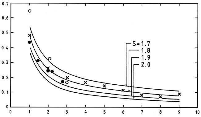Figure 7.1. Comparison between the observed left-hand side of Equation (7.1) (circles and crosses) and the theoretical right-hand side (solid lines) for a statistically homogeneous distribution of galaxies with a power-law two-point correlation function having exponent S (now usually denoted as ). (From Totsuji and Kihara 1969.) The y-axis is the value of Equation (7.1); the x-axis is angular separation on the sky.