6.2. Inflationary mechanisms

Different astrophysical objects, of different physical sizes, have comparable magnetic fields. This coincidence is hard to explain in the context of causal mechanisms of generation. The analogy with structure formation, already presented in the Introduction, is here useful. In the late seventies, prior to the formulation of the inflationary paradigm, the initial conditions for the density contrast were taken as primordial input. Later on, in the context of inflationary models, the primordial spectrum of curvature and density fluctuations could be calculated.

During inflation, in fact, fields of various spin are present and they can be excited by the dynamical evolution of the geometry. In the context of inflationary models of particular relevance are the scalar and tensor fluctuations of the geometry, corresponding respectively, to fluctuations of the scalar curvature and to gravitational waves. Gravitational waves and curvature perturbations obey evolution equations which are not invariant under Weyl rescaling of the four-dimensional metric. Then the quantum mechanical fluctuations in the corresponding fields will simply be amplified by the evolution of the background geometry.

It is interesting to speculate that large scale magnetic fields could be produced thanks to a similar mechanism. The major obstruction to this type of models is that gauge fields are not amplified thanks to the evolution of the background geometry the reason being that the evolution equations of gauge fields are invariant under Weyl rescaling of the metric.

When conformal invariance is broken, by some means, one is often led to estimate the amplitude of gauge field fluctuations arising as a result of the breaking. Clearly the detailed amount of amplified gauge fields will be specific of the particular model. In the following various ways of breaking conformal invariance will be listed without getting through the details of the calculations. Before doing so it is anyway instructive to introduce some general considerations stressing the analogy between the production of magnetic inhomogeneities and the production of gravitational inhomogeneities whose late time evolution leads the anisotropies in the CMB.

The tensor modes of the geometry are described by a rank-two (transverse and traceless) tensor in three spatial dimensions ⁽²⁵⁾, i.e.

(6.8)

obeying the equation, in Fourier space,

(6.9)

where µ_k = ah_k and h_k is the Fourier mode of each polarization. In this equation the "pump field" is simply given by the scale factor. When k² >> | a" / a| the mode is said to be adiabatically damped: in fact, in this regime, | h_k| a^-1, i.e. decreasing in an expanding Universe. In the opposite regime, i.e. k² << | a" / a| the mode is super-adiabatically amplified. In fact, during a de Sitter or quasi-de Sitter µ_k ~ a() and h_k is constant. Hence, for the whole time the given mode spends under the "potential barrier" of Eq. (6.9), it is amplified.

A similar equation holds for the canonical normal mode for the scalar fluctuations of the geometry, i.e.

(6.10)

The variable v_k is defined as

(6.11)

where _k is the fluctuation of the inflaton, _k is the curvature perturbation and is the scalar fluctuation of the geometry in the conformally Newtonian gauge [199, 200]. If the inflaton has an exponential potential z() a().

In the case of gauge fields, each of the two polarization of the appropriately rescaled vector potential obeys, the following equation

(6.12)

In specific models, g() may be associated with the gauge coupling. However g^-1() can also be viewed as a generic pump field arising as a result of the breaking of conformal invariance. The time dependence of the potential term is rather common to different models: it goes to zero for || as (² -1/4) ^-2. The numerical coefficient appearing in the potential determines the strength and spectrum of the amplified gauge fields whose subsequent evolution has to be however computed at finite conductivity.

In Fig. 6 the typical form of the potential term appearing in Eq. (6.12) is illustrated. Different comoving frequencies go under the barrier at different times and the amount of amplification is roughly proportional to the time spent under the barrier. Clearly, given the generic form of the barrier, smaller frequencies are more amplified than the frequencies comparable with the height of the barrier at ₁. In Fig. 6 the explicit numerical value of the height of the barrier corresponds to a (present) frequency of 10⁸ Hz which can be realized if the pump field goes to a constant right after the end of a conventional inflationary phase followed by a radiation-dominated stage of expansion.

Figure 6. The effective potential appearing in Eq. (6.12) is illustrated in general terms. In this example the pump field leading to amplification of electromagnetic quantum fluctuations is assumed to be constant prior to the onset of BBN. On the vertical axis few relevant physical frequencies (to be compared with the height of the potential) have been reported.

In the case of gravitational waves, and, with some caveats, in the case of scalar metric fluctuations, the "potential barriers" appearing, respectively, in Eqs. (6.9) and (6.10) may be related with the inverse Hubble radius. Hence, in the case of metric fluctuations, a mode which is under the barrier is also, with a swift terminology, outside the horizon (see Fig. 7). This is the reason why, following the conventional nomenclature, in Fig. 6 the moment when a given scale gets under the barrier has been denoted by _ex (i.e. horizon exit). According to the same convention, the moment when a given scale gets out the potential barrier is labeled by _re (i.e. horizon re-entry).

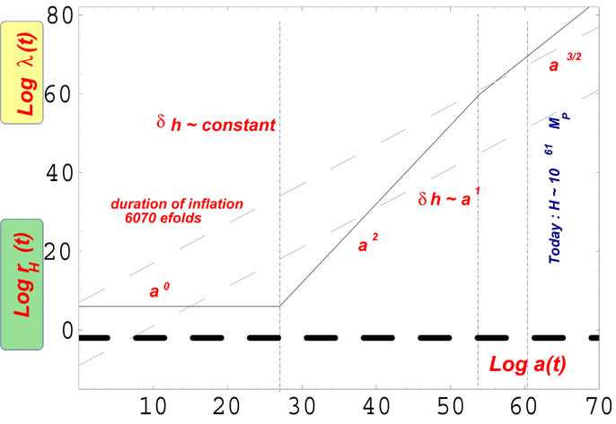Figure 7. The evolution of a given physical wavelength is illustrated in the case of an inflationary model with minimal duration. The region above the full curve (denoting the Hubble radius rH) = H-1) corresponds, for the tensor and scalar modes of the geometry, to the region where a given comoving wavenumber k is below the "potential barrier" appearing in Eqs. (6.9) and (6.10).

In Fig. 6 few relevant frequencies have been compared with the height of the barrier. Consider, for instance, _G i.e. the typical scale of gravitational collapse which is of the order of 1 Mpc, i.e. 10^-14 Hz. In Fig. 6 the physical frequency has been directly reported. Another interesting frequency is ~ mHz corresponding to the present value of the magnetic diffusivity momentum. The amplification caused by the parametric amplification of the vacuum fluctuations can be computed by solving Eq. (6.12) in the different regimes.

(6.13)

where ( C_k, D_k, and c_±(k) are integrations constants).

The mixing coefficients c_±(k), determining the parametric amplification of a mode k² < | V(₁)|, computed by matching these various branches of the solution reported in Eq. (6.13). One finds:

(6.14)

Similar calculations can be performed in order to obtain the spectrum of scalar and tensor fluctuations of the geometry [204, 205, 206].

Suppose now to make a simple estimate. Assume, for instance, that g is evolving prior to ₁ according to the dynamics dictated by a given model. Suppose also that after ₁ the Universe is suddenly dominated by radiation, and g' ~ 0 for > ₁. In this situation all the modes reenter during radiation and the amplification will be roughly given, to leading order by

(6.15)

If the function g() is identified with the evolving gauge coupling this result suggest that in order to have large amplification, g() has to grow from smaller to larger values. This is what happens, for instance, in the case of pre-big bang models where g ~ e^/2 and is the for-dimensional dilaton field [123].

Since we ought to estimate the amplification of an initial quantum mechanical fluctuations, a fully quantum mechanical treatment is certainly appropriate also in view of the discussion of the correlation properties of the obtained fluctuations. This analysis has been performed in [207] where the squeezing properties of the obtained photons have also been discussed.

The perturbed effective Lagrangian density

(6.16)

describes the evolution of the two ( = , ) transverse degrees of freedom defined by the Coulomb gauge condition A₀ = 0 and ^. = 0 (the prime denotes differentiation with respect to conformal time). The fields A = g have kinetic terms with canonical normalization and the time evolution given in Eq. (6.12) stems from the Euler-Lagrange equations derived from Eq. (6.16). By functionally deriving the the action the canonically conjugated momenta can be obtained leading to the Hamiltonian density and to the associated Hamiltonian

(6.17)

The operators corresponding to the classical polarizations appearing in the Hamiltonian density

(6.18)

obey canonical commutation relations and the associated creation and annihilation operators satisfy [_k,, ^†_p,] = ³( - ).

The (two-modes) Hamiltonian contains a free part and the effect of the variation of the coupling constant is encoded in the (Hermitian) interaction term which is quadratic in the creation and annihilation operators whose evolution equations, read, in the Heisenberg picture

(6.19)

The general solution of the previous system of equations can be written in terms of a Bogoliubov-Valatin transformation,

(6.20)

where _k,(0) = _k, and _-k, = _-k,. Notice that the Bogoliubov coefficients are the quantum analog of the mixing coefficients discussed in the semiclassical approach to the problem.

Unitarity requires that the two complex functions µ_k() and _k() are subjected to the condition |µ_k()|² - |_k()|² = 1 which also implies that µ_k() and _k() can be parameterized in terms of one real amplitude and two real phases

(6.21)

(r is sometimes called squeezing parameter and _k is the squeezing phase; from now on we will drop the subscript labeling each polarization if not strictly necessary). The total number of produced photons

(6.22)

is expressed in terms of _k = sin h² r_k, i.e. the mean number of produced photon pairs in the mode k. Inserting Eqs. (6.20)-(6.22) into Eqs. (6.19) we can derive a closed system involving only the _k and the related phases:

(6.23) (6.24) (6.25)

where f (_k) = [_k / (_k + 1)]^1/2.

In quantum optics [208, 209] the coherence properties of light fields have been a subject of intensive investigations for nearly half a century. In the present context the multiparticle states described so fare are nothing but squeezed states of the electromagnetic field [208, 209]. In fact, up to now the Heisenberg description has been adopted. In the Schrödinger picture the quantum mechanical states obtained as a result of the time evolution are exactly squeezed vacuum states [208, 209].

Magnetic fields over galactic scales have typical frequency of the order 10^-14-10^-15 Hz which clearly fall well outside the optical range. Thus, the analogy with quantum optics is only technical. The same quantum optical analogy has been successfully exploited in particle [210] and heavy-ions physics [211] of pion correlations (in order to measure the size of the strongly interacting region) and in the phenomenological analysis of hadronic multiplicity distributions.

The interference between the amplitudes of the magnetic fields (Young interferometry [212], in a quantum optical language) estimates the first order coherence of the magnetic background at different spatial locations making use of the two-point correlation function whose trace over the physical polarizations and for coincidental spatial locations is related to the magnetic energy density. Eqs. (6.23)-(6.25) can be solved once the pump field is specified but general expressions can be also obtained [207].

6.2.1. Conventional inflationary models

In conventional inflationary models it is very difficult to produce large scale magnetic fields with phenomenologically relevant strength. This potential difficulty has been scrutinized in various investigations [202, 213, 214, 215].

Turner and Widrow [213] listed a series of field theory models in de Sitter space with the purpose of finding a natural way of breaking conformal invariance. The first suggestion was that conformal invariance may be broken, at an effective level, through the coupling of photons to the geometry [216]. Typically, the breaking of conformal invariance occurs through products of gauge-field strengths and curvature tensors, i.e.

(6.26)

where m is the appropriate mass scale; R_µ and R_µ are the Riemann and Ricci tensors and R is the Ricci scalar. If the evolution of gauge fields is studied during a phase of de Sitter (or quasi-de Sittter) expansion, then the amplification of the vacuum fluctuations induced by the couplings listed in Eq. (6.26) is minute. The price in order to get large amplification should be, according to [213], an explicit breaking of gauge-invariance by direct coupling of the vector potential to the Ricci tensor or to the Ricci scalar, i.e.

(6.27)

In [213] two other different models were proposed (but not scrutinized in detail) namely scalar electrodynamics and the axionic coupling to the Abelian field strength.

Dolgov [215] considered the possible breaking of conformal invariance due to the trace anomaly. The idea is that the conformal invariance of gauge fields is broken by the triangle diagram where two photons in the external lines couple to the graviton through a loop of fermions. The local contribution to the effective action leads to the vertex ((-g)^1/2)¹⁺ F F where is a numerical coefficient depending upon the number of scalars and fermions present in the theory. The evolution equation for the gauge fields, can be written, in Fourier space, as

(6.28)

and it can be shown that only if > 0 the gauge fields are amplified. Furthermore, only is ~ 8 substantial amplification of gauge fields is possible.

In a series of papers [217, 218, 219] the possible effect of the axionic coupling to the amplification of gauge fields has been investigated. The idea is here that conformal invariance is broken through the explicit coupling of a pseudo-scalar field to the gauge field (see Section 5), i.e.

(6.29)

where is the dual field strength and where c is a numerical factor of order one. Consider now the case of a standard pseudoscalar potential, for instance m^{2 2}, evolving in a de Sitter (or quasi-de Sitter space-time). It can be shown, rather generically, that the vertex given in Eq. (6.29) leads to negligible amplification at large length-scales. The coupled system of evolution equations to be solved in order to get the amplified field is similar to Eqs. (5.123) already introduced in the duscussion of hypermagnetic fields

(6.30) (6.31)

From Eq. (6.30), there is a maximally amplified physical frequency

(6.32)

where the second equality follows from ~ a^-3/2 M cos mt (i.e. _max ~ m M). The amplification for ~ _max is of the order of exp[m_em / (2 H)] where H is the Hubble parameter during the de Sitter phase of expansion. From the above expressions one can argue that the modes which are substantially amplifed are the ones for which _max >> H. The modes interesting for the large-scale magnetic fields are the ones which are in the opposite range, i.e. _max << H. Clearly, by lowering the curvature scale of the problem the produced seeds may be larger and the conclusions much less pessimistic [219].

Another interesting idea pointed out by Ratra [214] is that the electromagnetic field may be directly coupled to the inflaton field. In this case the coupling is specified through a parameter , i.e. e F F where is the inflaton field in Planck units. In order to get sizable large-scale magnetic fields the effective gauge coupling must be larger than one during inflation (recall that is large, in Planck units, at the onset of inflation).

In [220] it has been suggested that the evolution of the Abelian gauge coupling during inflation induce the growth of the two-point function of magnetic inhomogeneities. This model is different from the one previously discussed [214]. Here the dynamics of the gauge coupling is not related to the dynamics of the inflaton which is not coupled to the Abelian field strength. In particular, r_B(Mpc) can be as large as 10^-12. In [220] the MHD equations have been generalized to the case of evolving gauge coupling. Recently a scenario similar to [220] has been discussed in [221].

In the perspective of generating large scale magnetic fields Gasperini [222] suggested to consider the possible mixing between the photon and the graviphoton field appearing in supergravity theories (see also, in a related context [223]). The graviphoton is the massive vector component of the gravitational supermultiplet and its interaction with the photon is specified by an interaction term of the type F_µ G^µ where G_µ is the filed strength of the massive vector. Large-scale magnetic fields with r_B(Mpc) 10^-34 can be obtained if ~ (1) and for a mass of the vector m ~ 10² TeV.

Bertolami and Mota [224] argue that if Lorentz invariance is spontaneously broken, then photons acquire naturally a coupling to the geometry which is not gauge-invariant and which is similar to the coupling considered in [213].

Finally Davis and Dimopoulos [225] considered the possibility of phase transitions taking place during inflation. They found that sizable large-scale magnetic fields can be generated provided the phase transition occurs in the last 5 e-foldings of the inflationary stage of expansion.

6.2.2. Abelian Higgs model

While the coupling of electromagnetic field to the metric and to the charged fields is conformally invariant, the coupling of the charged scalar field to gravity is not. Thus, vacuum fluctuations of the charged scalar field can be amplified during inflation at super-horizon scales, leading potentially to non-trivial correlations of the electric currents and charges over cosmological distances. The fluctuations of electric currents, in turn, may induce magnetic fields through Maxwell equations at the corresponding scales. The role of the charged scalar field may be played by the Higgs boson which couples to the hypercharge field above the electroweak phase transition; the generated hypercharged field is converted into ordinary magnetic field at the temperatures of the order of electroweak scale.

No detailed computations were carried out in [213] in order to substantiate this idea. The suggestion of [213] was further developed quite recently in [226] for the standard electroweak theory with an optimistic conclusion that large scale magnetic fields can be indeed generated. In [227] a supersymmetric model was studied. In [134], previous treatments have been further scrutinized by computing, with higher accuracy, the amplification of the charged scalar field and the damping induced by the conductivity. It turns out that the resulting magnetic fields are insufficient in order to provide reasonable seeds for the dynamo amplification.

Introducing appropriately rescaled fields the action of the Abelian-Higgs model in a conformally flat FRW space-time can be written as

(6.33)

Now, since the evolution equation of the charged scalar is not conformally invariant, current density and charge density fluctuations will be induced. Then, by employing a Vlasov-Landau description similar to the one introduced in Section 5, the resulting magnetic field will be of the order of B_dec ~ 10^-40 T_dec² which is, by far, too small. Later it has been proposed that much larger magnetic fields may be obtained in the context of the Abelian-Higgs model [228] (see however [229] for a detailed criticism of this proposal).

6.2.3. Internal dimensions

If internal dimensions are dynamical, then Weyl invariance may be naturally broken [230]. Consider a pure electromagnetic fluctuation decoupled from the sources, representing an electromagnetic wave propagating in the d-dimensional external space such that A_µ A_µ(, ), A_a = 0. In the metric given in Eq. (5.1) the evolution equation of the gauge field fluctuations can be written as

(6.34)

where F = _[ A_] is the gauge field strength and G is the determinant of the D dimensional metric. Notice that if n = 0 the space-time is isotropic and, therefore, the Maxwell's equations can be reduced (by trivial rescaling) to the flat space equations. If n 0 we have that the evolution equation of the electromagnetic fluctuations propagating in the external d-dimensional manifold will receive a contribution from the internal dimensions which cannot be rescaled away [233] ⁽²⁶⁾. In the radiation gauge (A₀ = 0 and _i Aⁱ = 0) ⁽²⁷⁾ the evolution the vector potentials can be written as

(6.35)

The vector potentials A_i are already rescaled with respect to the (conformally flat) d + 1 dimensional metric. In terms of the canonical normal modes of oscillations _i = b^n/2 A_i the previous equation can be written in a simpler form, namely

(6.36)

In order to estimate the amplification of the gauge fields induced by the evolution of the internal geometry we shall consider the background metric of Eq. (5.13) in the case of maximally symmetric subspaces _ij = _ij, _ab = _ab.

Suppose now that the background geometry evolves along three different epochs. During the first phase (taking place for ] - , - ₁]) the evolution is truly multidimensional. At = - ₁ the multidimensional dynamics is continuously matched to a radiation dominated phase turning, after decoupling, into a matter dominated regime of expansion. During the radiation and matter dominated stages the internal dimensions are fixed to their (present) constant size in order not to conflict with possible bounds arising both at the BBN time and during the matter-dominated epoch. The evolution of the external dimensions does not affect the amplification of the gauge fields as it can be argued from Eq. (6.36) :in the limit n 0 (i.e. conformally invariant background) Eq. (6.36) reduces to the flat space equation. A background with the features described above has been introduced in Eq. (5.14).

Defining, respectively, b_BBN and b₀ as the size of the internal dimensions at the BBN time and at the present epoch, the maximal variation allowed to the internal scale factor from the BBN time can be expressed as b_BBN / b₀ ~ 1 + where || < 10^-2 [116, 117, 118]. The bounds on the variation of the internal dimensions during the matter dominated epoch are even stronger. Denoting with an over-dot the derivation with respect to the cosmic time coordinate, we have that | / b| < 10^-9H₀ where H₀ is the present value of the Hubble parameter [116]. The fact that the time evolution of internal dimensions is so tightly constrained for temperatures lower of 1 MeV does not forbid that they could have been dynamical prior to that epoch [231].

In the parameterization of Eq. (5.14) the internal dimensions grow (in conformal time) for < 0 and they shrink ⁽²⁸⁾ for > 0.

By inserting this background into Eq. (6.36) we obtain that for < - ₁

(6.37)

whereas V() 0 for > - ₁. Since V() goes to zero for ± we can define, in both limits, a Fourier expansion of _i in terms of two distinct orthonormal sets of modes. The amplification of the quantum mechanical fluctuations of the gauge fields can then be computed using the standard techniques (see, for instance, [234, 235, 236]). In [230] it has been shown that in simple models of dimensional decoupling magnetic fields can be generated with strength compatible with the bound of Eq. (6.2). In particular there is the interesting possibility that large-scale magnetic fields are produced in the case when internal dimensions also expand while the external ones also expand but at a different rate.

It should be mentioned that the interplay between gauge fields and large (or infinite) extra-dimensions is still under investigation. There is, at the moment, no definite model leading to the generation of large-scale magnetic field in a framework of infinite internal dimensions. The main reason is that it is difficult to build reasonable cosmological models with large extra-dimensions. More specifically, one would like to have a model where gauge fields arise naturally in the bulk. In six- dimensions interesting models can be constructed [239] where localized gauge zero modes may be naturally present (in analogy with what happens in the case of six-dimensional warped models [240, 241]).

6.2.4. String cosmological models

Large scale magnetic fields may also be produced in the context of string cosmological models [202, 289] (see also [238] for the analysis of the amplification of magnetic fields during a phase of coherent dilaton oscillations ⁽²⁹⁾). In many respects the case of string cosmological models is related to the one where the gauge coupling is dynamical. However, in the string cosmological context, the dynamics of the gauge coupling and of the geometry are connected by the solutions of the low-energy -functions. The basic evolution of the background and of the gauge coupling has been discussed in Section 5. In order to achieve a large amplification of the quantum fluctuations of the gauge fields, the gauge coupling should be sufficiently small when the typical scale of the gravitational collapse hits the "potential barrier". In particular, g_ex(_G) < 10^-33 is the dynamo requirement has to be satisfied. It is difficult to produce large scale magnetic fields with reasonable amplitudes if the pre-big bang phase matches immediately to the post-big bang evolution [237]. However, phenomenologically consistent pre-big bang models lead to a sufficiently long stringy phase when the dilaton and the curvature scale are roughly constant. If this phase is included the conditions expressed by Eqs. (6.1) and (6.2) are easily satisfied. Furthermore, there are regions in the parameter space of the model where r_B(_G) ~ 10^-8 which implies that the galactic magnetic field may be fully primordial [202, 289], i.e. no dynamo action will be required.

²⁵ The theory of cosmological perturbations is assumed in the following considerations. Comprehensive accounts of the relevant topics can be found in [199, 200] (see also [201]). Back.

²⁶ Notice that the electromagnetic field couples only to the internal dimensions through the determinant of the D-dimensional metric. In string theories, quite generically, the one-form fields are also coupled to the dilaton field. This case has been already analyzed in the context of string inspired cosmological scenarios and will be discussed later. Back.

²⁷ For a discussion of gauges in curved spaces see [232]. Back.

²⁸ To assume that the internal dimensions are constant during the radiation and matter dominated epoch is not strictly necessary. If the internal dimensions have a time variation during the radiation phase we must anyway impose the BBN bounds on their variation [116, 117, 118] . The tiny variation allowed by BBN implies that b() must be effectively constant for practical purposes. Back.

²⁹ The possible production of (short scale) magnetic fields by parametric resonance explored in [238] , has been subsequently analyzed in the standard inflationary contex [203] Back.