Annu. Rev. Astron. Astrophys. 2002. 40: 171-216 Copyright © 2002 by Annual Reviews. All rights reserved

5. DATA ANALYSIS

The very large CMB data sets that have begun arriving require new, innovative tools of analysis. The fundamental tool for analyzing CMB data - the likelihood function - has been used since the early days of anisotropy searches [Readhead et al, 1989, Bond et al, 1991, Dodelson & Jubas, 1993]. Brute force likelihood analyses [Tegmark & Bunn, 1995] were performed even on the relatively large COBE data set, with six thousand pixels in its map. Present data sets are a factor of ten larger, and this factor will soon get larger by yet another factor of a hundred. The brute force approach, the time for which scales as the number of pixels cubed, no longer suffices.

In response, analysts have devised a host of techniques that move beyond the early brute force approach. The simplicity of CMB physics - due to linearity - is mirrored in analysis by the apparent Gaussianity of both the signal and many sources of noise. In the Gaussian limit, optimal statistics are easy to identify. These compress the data so that all of the information is retained, but the subsequent analysis - because of the compression - becomes tractable.

The Gaussianity of the CMB is not shared by other cosmological systems since gravitational non-linearities turn an initially Gaussian distribution into a non-Gaussian one. Nontheless, many of the techniques devised to study the CMB have been proposed for studying: the 3D galaxy distribution [Tegmark et al, 1998], the 2D galaxy distribution [Efstathiou & Moody, 2001, Huterer et al, 2001] the Lyman alpha forest [Hui et al, 2001], the shear field from weak lensing [Hu & White, 2001], among others. Indeed, these techniques are now indispensible, powerful tools for all cosmologists, and we would be remiss not to at least outline them in a disussion of the CMB, the context in which many of them were developed.

Figure 5 summarizes the path from the data analyis starting point, a timestream of data points, to the end, the determination of cosmological parameters. Preceding this starting point comes the calibration and the removal of systematic errors from the raw data, but being experiment specific, we do not attempt to cover such issues here. ⁴ Each step radically compresses the data by reducing the number of parameters used to describe it. Although this data pipeline and our discussion below are focused on temperature anisotropies, similar steps have been elucidated for polarization [Bunn, 2001, Tegmark & de Oliveira-Costa, 2001, Lewis et al, 2001].

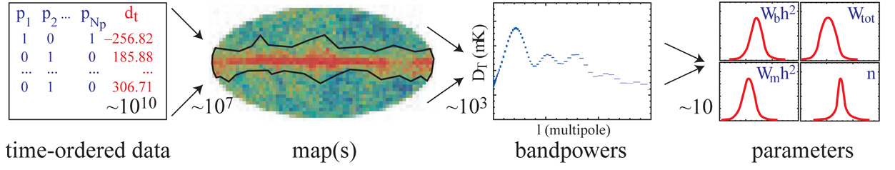Figure 5. Data pipeline and radical compression. Map are constructed for each frequency channel from the data timestreams, combined and cleaned of foreground contamination by spatial (represented here by excising the galaxy) and frequency information. Bandpowers are extracted from the maps and cosmological parameters from the bandpowers. Each step involves a substantial reduction in the number of parameters needed to describe the data, from potentially 1010 10 for the Planck satellite.

5.1. Mapmaking

An experiment can be characterized by the data d_t taken at many different times; a pointing matrix P_ti, relating the data timestream to the underlying signal at pixelized positions indexed by i, and a noise matrix C_{d, tt'} characterizing the covariance of the noise in the timestream. A model for the data then is d_t = P_{ti i} + n_t (with implicit sum over the repeating index i); it is the sum of signal plus noise. Here n_t is drawn from a distribution (often Gaussian) with mean zero and covariance <n_t n_t'> = C_{d, tt'}. In its simplest form the pointing matrix P contains rows - which corresponds to a particular time - with all zeroes in it except for one column with a one (see Figure 5). That column corresponds to the particular pixel observed at the time of interest. Typically, a pixel will be scanned many times during an experiment, so a given column will have many ones in it, corresponding to the many times the pixel has been observed.

Given this model, a well-posed question is: what is the optimal estimator for the signal _i? i.e. what is the best way to construct a map? The answer stems from the likelihood function , defined as the probability of getting the data given the theory P[data| theory]. In this case, the theory is the set of parameters _i,

(26)

That is, the noise, the difference between the data and the modulated signal, is assumed to be Gaussian with covariance C_d.

There are two important theorems useful in the construction of a map and more generally in each step of the data pipeline [Tegmark et al, 1997]. The first is Bayes' Theorem. In this context, it says that P[_i| d_t], the probability that the temperatures are equal to _i given the data, is proportional to the likelihood function times a prior P(_i). Thus, with a uniform prior,

(27)

with the normalization constant determined by requiring the integral of the probability over all _i to be equal to one. The probability on the left is the one of interest. The most likely values of _i therefore are those which maximize the likelihood function. Since the log of the likelihood function in question, Equation (26), is quadratic in the parameters _i, it is straightforward to find this maximum point. Differentiating the argument of the exponential with respect to _i and setting to zero leads immediately to the estimator

(28)

where C_N (P^tr C_d^-1 P)^-1. As the notation suggests, the mean of the estimator is equal to the actual _i and the variance is equal to C_N.

The second theorem states that this maximum likelihood estimator is also the minimum variance estimator. The Cramer-Rao inequality says no estimator can measure the _i with errors smaller than the diagonal elements of F^-1, where the Fisher matrix is defined as

(29)

Inspection of Equation (26) shows that, in this case the Fisher matrix is precisely equal to C_N^-1. Therefore, the Cramer-Rao theorem implies that the estimator of Equation (28) is optimal: it has the smallest possible variance [Tegmark, 1997a]. No information is lost if the map is used in subsequent analysis instead of the timestream data, but huge factors of compression have been gained. For example, in the recent Boomerang experiment [Netterfield et al, 2001], the timestream contained 2 × 10⁸ numbers, while the map had only 57, 000 pixels. The map resulted in compression by a factor of 3500.

There are numerous complications that must be dealt with in realistic applications of Equation (28). Perhaps the most difficult is estimation of C_d, the timestream noise covariance. This typically must be done from the data itself [Ferreira & Jaffe, 2000, Stompor et al, 2001]. Even if C_d were known perfectly, evaluation of the map involves inverting C_d, a process which scales as the number of raw data points cubed. For both of these problems, the assumed stationarity of C_{d, tt'} (it depends only on t - t') is of considerable utility. Iterative techniques to approximate matrix inversion can also assist in this process [Wright et al, 1996]. Another issue which has received much attention is the choice of pixelization. The community has converged on the Healpix pixelization scheme ⁵, now freely available.

Perhaps the most dangerous complication arises from astrophysical foregrounds, both within and from outside the Galaxy, the main ones being synchrotron, bremmsstrahlung, dust and point source emission. All of the main foregrounds have different spectral shapes than the blackbody shape of the CMB. Modern experiments typically observe at several different frequencies, so a well-posed question is: how can we best extract the CMB signal from the different frequency channels [Bouchet & Gispert, 1999]? The blackbody shape of the CMB relates the signal in all the channels, leaving one free parameter. Similarly, if the foreground shapes are known, each foreground comes with just one free parameter per pixel. A likelihood function for the data can again be written down and the best estimator for the CMB amplitude determined analytically. While in the absence of foregrounds, one would extract the CMB signal by weighting the frequency channels according to inverse noise, when foregrounds are present, the optimal combination of different frequency maps is a more clever weighting that subtracts out the foreground contribution [Dodelson, 1997]. One can do better if the pixel-to-pixel correlations of the foregrounds can also be modeled from power spectra [Tegmark & Efstathiou, 1996] or templates derived from external data.

This picture is complicated somewhat because the foreground shapes are not precisely known, varying across the sky, e.g. from a spatially varying dust temperature. This too can be modelled in the covariance and addressed in the likelihood [Tegmark, 1998, White, 1998]. The resulting cleaned CMB map is obviously noisier than if foregrounds were not around, but the multiple channels keep the degradation managable. For example, the errors on some cosmological parameters coming from Planck may degrade by almost a factor of ten as compared with the no-foreground case. However, many errors will not degrade at all, and even the degraded parameters will still be determined with unprecedented precision [Knox, 1999, Prunet et al, 2000, Tegmark et al, 2000].

Many foregrounds tend to be highly non-Gaussian and in particular well-localized in particular regions of the map. These pixels can be removed from the map as was done for the region around the galactic disk for COBE. This technique can also be highly effective against point sources. Indeed, even if there is only one frequency channel, external foreground templates set the form of the additional contributions to C_N, which, when properly included, immunize the remaining operations in the data pipeline to such contaminants [Bond et al, 1998]. The same technique can be used with templates of residual systematics or constraints imposed on the data, from e.g. the removal of a dipole.

5.2. Bandpower Estimation

Figure 5 indicates that the next step in the compression process is extracting bandpowers from the map. What is a bandpower and how can it be extracted from the map? To answer these questions, we must construct a new likelihood function, one in which the estimated _i are the data. No theory predicts an individual _i, but all predict the distribution from which the individual temperatures are drawn. For example, if the theory predicts Gaussian fluctuations, then _i is distributed as a Gaussian with mean zero and covariance equal to the sum of the noise covariance matrix C_N and the covariance due to the finite sample of the cosmic signal C_S. Inverting Equation (1) and using Equation (2) for the ensemble average leads to

(30)

where _T, depends on the theoretical parameters through C (see Equation (3)). Here W, the window function, is proportional to the Legendre polynomial P(_i ^. _j) and a beam and pixel smearing factor b². For example, a Gaussian beam of width , dictates that the observed map is actually a smoothed picture of true signal, insensitive to structure on scales smaller than . If the pixel scale is much smaller than the beam scale, b² e^-(+1)2. Techniques for handling asymmetric beams have also recently been developed [Wu et al, 2001, Wandelt & Gorski, 2001, Souradeep & Ratra, 2001]. Using bandpowers corresponds to assuming that _T, is constant over a finite range, or band, of , equal to B_a for _a - _a / 2 < < _a + _a / 2. Plate 1 gives a sense of the width and number of bands N_b probed by existing experiments.

For Gaussian theories, then, the likelihood function is

(31)

where C = C_S + C_N and N_p is the number of pixels in the map. As before, _B is Gaussian in the anisotropies _i, but in this case _i are not the parameters to be determined; the theoretical parameters are the B_a, upon which the covariance matrix depends. Therefore, the likelihood function is not Gaussian in the parameters, and there is no simple, analytic way to find the point in parameter space (which is multi-dimensional depending on the number of bands being fit) at which _B is a maximum. An alternative is to evaluate _B numerically at many points in a grid in parameter space. The maximum of the _B on this grid then determines the best fit values of the parameters. Confidence levels on say B₁ can be determined by finding the region within which _a^b dB₁ [_i=2^N_b d^B_i] _B = 0.95, say, for 95% limits.

This possibility is no longer viable due to the sheer volume of data. Consider the Boomerang experiment with N_p = 57, 000. A single evaluation of _B involves computation of the inverse and determinant of the N_p × N_p matrix C, both of which scale as N_p³. While this single evaluation might be possible with a powerful computer, a single evaluation does not suffice. The parameter space consists of N_b = 19 bandpowers equally spaced from l_a = 100 up to l_a = 1000. A blindly placed grid on this space would require at least ten evaluations in each dimension, so the time required to adequately evaluate the bandpowers would scale as 10¹⁹ N_p³. No computer can do this. The situation is rapidly getting worse (better) since Planck will have of order 10⁷ pixels and be sensitive to of order a 10³ bands.

It is clear that a "smart" sampling of the likelihood in parameter space is necessary. The numerical problem, searching for the local maximum of a function, is well-posed, and a number of search algorithms might be used. _B tends to be sufficiently structureless that these techniques suffice. [Bond et al, 1998] proposed the Newton-Raphson method which has become widely used. One expands the derivative of the log of the likelihood function - which vanishes at the true maximum of _B - around a trial point in parameter space, B_a⁽⁰⁾. Keeping terms second order in B_a - B_a⁽⁰⁾ leads to

(32)

where the curvature matrix _B,ab is the second derivative of -ln _B with respect to B_a and B_b. Note the subtle distinction between the curvature matrix and the Fisher matrix in Equation (29), F = <>. In general, the curvature matrix depends on the data, on the _i. In practice, though, analysts typically use the inverse of the Fisher matrix in Equation (32). In that case, the estimator becomes

(33)

quadratic in the data _i. The Fisher matrix is equal to

(34)

In the spirit of the Newton-Raphson method, Equation (33) is used iteratively but often converges after just a handful of iterations. The usual approximation is then to take the covariance between the bands as the inverse of the Fisher matrix evaluated at the convergent point C_B = F_B^-1. Indeed, [Tegmark, 1997b] derived the identical estimator by considering all unbiased quadratic estimators, and identifying this one as the one with the smallest variance.

Although the estimator in Equation (33) represents a ~ 10^N_b improvement over brute force coverage of the parameter space - converging in just several iterations - it still requires operations which scale as N_p³. One means of speeding up the calculations is to transform the data from the pixel basis to the so-called signal-to-noise basis, based on an initial guess as to the signal, and throwing out those modes which have low signal-to-noise [Bond, 1995, Bunn & Sugiyama, 1995]. The drawback is that this procedure still requires at least one N_p³ operation and potentially many as the guess at the signal improves by iteration. Methods to truly avoid this prohibitive N_p³ scaling [Oh et al, 1999, Wandelt & Hansen, 2001] have been devised for experiments with particular scan strategies, but the general problem remains open. A potentially promising approach involves extracting the real space correlation functions as an intermediate step between the map and the bandpowers [Szapudi et al, 2001]. Another involves consistently analyzing coarsely pixelized maps with finely pixelized sub-maps [Dore et al, 2001].

5.3. Cosmological Parameter Estimation

The huge advantage of bandpowers is that they represent the natural meeting ground of theory and experiment. The above two sections outline some of the steps involved in extracting them from the observations. Once they are extracted, any theory can be compared with the observations without knowledge of experimental details. The simplest way to estimate the cosmological parameters in a set c_i is to approximate the likelihood as

(35)

and evaluate it at many points in parameter space (the bandpowers depend on the cosmological parameters). Since the number of cosmological parameters in the working model is N_c ~ 10 this represents a final radical compression of information in the original timestream which recall has up to N_t ~ 10¹⁰ data points.

In the approximation that the band power covariance C_B is independent of the parameters c, maximizing the likelihood is the same as minimizing ². This has been done by dozens of groups over the last few years especially since the release of CMBFAST [Seljak & Zaldarriaga, 1996], which allows fast computation of theoretical spectra. Even after all the compression summarized in Figure 5, these analyses are still computationally cumbersome due to the large numbers of parameters varied. Various methods of speeding up spectra computation have been proposed [Tegmark & Zaldarriaga, 2000], based on the understanding of the physics of peaks outlined in Section 3, and Monte Carlo explorations of the likelihood function [Christensen et al, 2001].

Again the inverse Fisher matrix gives a quick and dirty estimate of the errors. Here the analogue of Equation (29) for the cosmological parameters becomes

(36)

In fact, this estimate has been widely used to forecast the optimal errors on cosmological parameters given a proposed experiment and a band covariance matrix C_B which includes diagonal sample and instrumental noise variance. The reader should be aware that no experiment to date has even come close to achieving the precision implied by such a forecast!

As we enter the age of precision cosmology, a number of caveats will become increasingly important. No theoretical spectra are truly flat in a given band, so the question of how to weight a theoretical spectrum to obtain B_a can be important. In principle, one must convolve the theoretical spectra with window functions [Knox, 1999] distinct from those in Equation (30) to produce B_a. Among recent experiments, DASI [Pryke et al, 2001] among others have provided these functions. Another complication arises since the true likelihood function for B_a is not Gaussian, i.e. not of the form in Equation (35). The true distribution is skewed: the cosmic variance of Equation (4) leads to larger errors for an upward fluctuation than for a downward fluctuation. The true distribution is closer to log-normal [Bond et al, 2000], and several groups have already accounted for this in their parameter extractions.

⁴ Aside from COBE, experiments to date have had a sizable calibration error (~ 5-10%) which must be factored into the interpretation of Plate 1. Back.

⁵ http://healpix.jpl.nasa.gov/ Back.