Copyright © 2001 by Annual Reviews. All rights reserved
| Annu. Rev. Astron. Astrophys. 2001. 39:
137-174 Copyright © 2001 by Annual Reviews. All rights reserved |


Although the mathematics of rotating disks is well established (e.g., Plummer 1911, Mestel, 1963, Toomre 1982, Binney & Tremaine 1987, Binney & Merrifield, 1998) the analysis of the observational data has continued to evolve as the quality of the data has improved. Both emission lines and absorption lines at a point on a spectrum are an integral along the line of sight through the galaxy. Only recently has the quality of the observational material permitted the deconvolution of various components. We describe a few procedures below.
3.1. Intensity-Weighted-Velocity Method
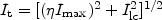
A rotation curve of a galaxy is defined as the trace of velocities on a position-velocity (PV) diagram along the major axis, corrected for the angle between the line-of-sight and the galaxy disk. A widely used method is to trace intensity-weighted velocities (Warner et al. 1973), which are defined by
 |
(1) |
where I(v) is the intensity profile at a given radius as a function of the radial velocity. Rotation velocity is then given by
 |
(2) |
where i is the inclination angle and Vsys is the systemic velocity of the galaxy.
3.2. Centroid-Velocity and Peak-Intensity-Velocity Methods
In outer galactic disks, where line profiles can be assumed to be symmetric about the peak-intensity value, the intensity-weighted velocity can be approximated by a centroid velocity of half-maximum values of a line profile (Rubin et al. 1980, 1982, 1985), or alternatively by a velocity at which the intensity attains its maximum, the peak-intensity velocity (Mathewson et al. 1992, 1996). Both methods have been adopted in deriving emission line rotation curves. Tests indicate that centroid measures of weak emission lines show less scatter (Rubin, unpublished).
However, for inner regions, where the line profiles are not simple, but are superposition of outer and inner disk components, these two methods often under-estimate the true rotation velocity. The same situation occurs for edge-on galaxies, where line profiles are the superposition of profiles arising from all radial distances sampled along the line-of-sight. In these circumstances, the envelope-tracing method described below gives more reliable rotation curves.
This method makes use of the terminal velocity in a PV diagram along the major axis. The rotation velocity is derived by using the terminal velocity Vt:
 |
(3) |
where  ISM and
obs are
the velocity dispersion of the interstellar gas and the velocity resolution
of observations, respectively.
The interstellar velocity dispersion is of the order of
ISM ~ 7 to 10
km s-1, while
obs depends on
instruments.
ISM and
obs are
the velocity dispersion of the interstellar gas and the velocity resolution
of observations, respectively.
The interstellar velocity dispersion is of the order of
ISM ~ 7 to 10
km s-1, while
obs depends on
instruments.
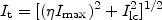
Here, the terminal velocity is defined by a velocity at which the intensity becomes equal to
 |
(4) |
on observed PV diagrams, where
Imax and Ilc are
the maximum intensity and intensity corresponding to the lowest contour
level, respectively, and
 is usually
taken to be 0.2 to 0.5.
For = 0.2,
this equation defines a 20% level of the intensity profile at a fixed
position,
It
is usually
taken to be 0.2 to 0.5.
For = 0.2,
this equation defines a 20% level of the intensity profile at a fixed
position,
It  0.2 × Imax,
if the signal-to-noise ratio is sufficiently high. If the intensity is
weak, the equation gives
It
Ilc which approximately defines the loci along
the lowest contour level (usually ~ 3 × rms noise).
0.2 × Imax,
if the signal-to-noise ratio is sufficiently high. If the intensity is
weak, the equation gives
It
Ilc which approximately defines the loci along
the lowest contour level (usually ~ 3 × rms noise).
For nearly face-on galaxies observed at sufficiently high angular resolution, these three methods give an almost identical rotation curve. However, both finite beam width and disk thickness along the line of sight cause confusion of gas with smaller velocities than the terminal velocity, which often results in a lower rotation velocity in the former two methods.
The envelope-tracing method is ill-defined when applied to the innermost part of a PV diagram, for the two sides of the nucleus have a discontinuity at the nucleus due principally to the instrumental resolution, which is large with respect to the velocity gradients. In practice, this discontinuity is avoided by stopping the tracing at a radius corresponding to the telescope resolution, and then approximating the rotation curve by a straight line crossing the nucleus at zero velocity. The "solid body" rotation implied by this procedure is probably a poor approximation to the true motions near the nucleus (Section 4.3).
Takamiya and Sofue (private communication) have developed an iterative method to derive a rotation curve. This extremely reliable method comprises the following procedure. An initial rotation curve, RC0, is adopted from a PV diagram (PV0), obtained by any method as above (e.g. a peak-intensity method). Using this rotation curve and an observed radial distribution of intensity (emissivity) of the line used in the analysis, a PV diagram, PV1, is constructed. The difference between this calculated PV diagram and the original PV0, e.g. the difference between peak-intensity velocities, is used to correct the initial rotation curve to obtain a corrected rotation curve, RC1. This RC is used to calculated another PV diagram PV2 using the observed intensity distribution, and to obtain the next iterated rotation curve, RC2 by correcting for the difference between PV2 and PV0. This iteration is repeated until PVi and PV0 becomes identical, such that the summation of root mean square of the differences between PVi and PV0 becomes minimum and stable. RCi is adopted as the most reliable rotation curve.
3.5. Absorption Line Velocities
For several decades, the Fourier quotient technique (Simkin 1974, Sargent et al. 1977) or the correlation technique (Bender 1990, Franx & Illingworth 1988) were methods of choice for determining rotation velocities within early-type galaxies. Both procedures assume that the stellar absorption lines formed by the integration along the line of sight through the galaxy can be fit by a Gaussian profile. However, recent instrumental improvements confirm that even disk galaxies consist of multi-component kinematic structures, so more sophisticated methods of analysis are required to reveal velocity details of the separate stellar components.
Various methods have been devised to account for the non-Gaussian form of the line-of-sight velocity distribution. Line profiles can be expanded into a truncated Gauss-Hermite series (van der Marel & Franx 1993) which measure the asymmetric deviations (h3) and the symmetric deviations (h4) from Gaussian. Alternatively, one can use the unresolved Gaussian decomposition method (Kuijken and Merrifield 1993). Other procedures to determine line profiles and their higher order moments (e.g. Bender 1990, Rix & White 1992, Gerhard 1993) are in general agreement (Fisher 1997); differences arise from signal-to-noise, resolution, and template mismatch. Such procedures will define the future state-of-the-art.
3.6. Dependence on Observational Methods
Disk galaxies are a complex combination of various structural components. Observations from emission lines and absorption lines in the optical, mm, and radio regions may not sample identical regions along the same line-of-sight. Instruments sample at different sensitivities with different wavelength and spatial resolutions. Results are a function of the techniques of observations and reductions. A simple "rotation curve" is an approximation as a function of radius to the full velocity field of a disk galaxy. As such, it can be obtained only by neglecting small scale velocity variations, and by averaging and smoothing rotation velocities from both sides of the galactic center. Because it is a simple, albeit approximate, description of a spiral velocity field, it is likely to be valuable even as more complex descriptions become available for many galaxies.