


The modern physical description of the Universe as a whole can be traced back to Einstein, who argued theoretically for the so-called "cosmological principle": that the distribution of matter and energy must be homogeneous and isotropic on the largest scales. Today isotropy is well established (see the review by Wu, Lahav, & Rees 1999 [389]) for the distribution of faint radio sources, optically-selected galaxies, the X-ray background, and most importantly the cosmic microwave background (hereafter, CMB; see, e.g., Bennett et al. 1996 [36]). The constraints on homogeneity are less strict, but a cosmological model in which the Universe is isotropic but significantly inhomogeneous in spherical shells around our special location, is also excluded [155].
In General Relativity, the metric for a space which is spatially homogeneous and isotropic is the Friedman-Robertson-Walker metric, which can be written in the form
 |
(1) |
where a(t) is
the cosmic scale factor which describes expansion in time, and
(R,  ,
,
 ) are spherical
comoving coordinates. The constant k
determines the geometry of the metric; it is positive in a closed Universe,
zero in a flat Universe, and negative in an open Universe. Observers at
rest remain at rest, at fixed (R,
,
), with their
physical separation increasing with time in proportion to
a(t). A given observer
sees a nearby observer at physical distance D receding at the Hubble
velocity H(t)D, where the Hubble constant at time
t is
H(t) = d a(t) / dt. Light
emitted by a source at time t is observed at
t = 0 with a redshift z = 1/a(t) - 1, where
we set a(t = 0)
) are spherical
comoving coordinates. The constant k
determines the geometry of the metric; it is positive in a closed Universe,
zero in a flat Universe, and negative in an open Universe. Observers at
rest remain at rest, at fixed (R,
,
), with their
physical separation increasing with time in proportion to
a(t). A given observer
sees a nearby observer at physical distance D receding at the Hubble
velocity H(t)D, where the Hubble constant at time
t is
H(t) = d a(t) / dt. Light
emitted by a source at time t is observed at
t = 0 with a redshift z = 1/a(t) - 1, where
we set a(t = 0)
 1
for convenience (but note that old textbooks may use a different
convention).
1
for convenience (but note that old textbooks may use a different
convention).
The Einstein field equations of General Relativity yield the Friedmann equation (e.g., Weinberg 1972 [376]; Kolb & Turner 1990 [205])
 |
(2) |
which relates the expansion of the Universe to its matter-energy
content. For each component of the energy density
 , with an
equation of state p =
p(), the
density varies
with a(t) according to the equation of energy conservation
, with an
equation of state p =
p(), the
density varies
with a(t) according to the equation of energy conservation
 |
(3) |
With the critical density
 |
(4) |
defined as the density needed for k = 0, we define the ratio of the total density to the critical density as
 |
(5) |
With  m,
m,
 ,
and r
denoting the present contributions
to from matter
(including cold dark matter as well as a contribution
b from
baryons), vacuum density (cosmological
constant), and radiation, respectively, the Friedmann equation becomes
,
and r
denoting the present contributions
to from matter
(including cold dark matter as well as a contribution
b from
baryons), vacuum density (cosmological
constant), and radiation, respectively, the Friedmann equation becomes
 |
(6) |
where we define H0 and
0 =
m +
+
r to be
the present values of H and
,
respectively, and we let
 |
(7) |
In the particularly simple Einstein-de Sitter model
(m = 1,
=
r =
k = 0),
the scale factor varies as a(t)
 t2/3. Even models with non-zero
or
k
approach the Einstein-de Sitter behavior at high redshift, i.e. when (1
+ z) >>
|m-1 - 1| (as long as
r can be
neglected). In this high-z regime the age of the Universe is,
t2/3. Even models with non-zero
or
k
approach the Einstein-de Sitter behavior at high redshift, i.e. when (1
+ z) >>
|m-1 - 1| (as long as
r can be
neglected). In this high-z regime the age of the Universe is,
 |
(8) |
The Friedmann equation implies that models with
k = 0
converge to the Einstein-de Sitter limit faster than do open models.
In the standard hot Big Bang model, the Universe is initially hot and the energy density is dominated by radiation. The transition to matter domination occurs at z ~ 3500, but the Universe remains hot enough that the gas is ionized, and electron-photon scattering effectively couples the matter and radiation. At z ~ 1100 the temperature drops below ~ 3000K and protons and electrons recombine to form neutral hydrogen. The photons then decouple and travel freely until the present, when they are observed as the CMB [348].
3.2. Composition of the Universe
According to the standard cosmological model, the Universe started at the big bang about 14 billion years ago. During an early epoch of accelerated superluminal expansion, called inflation, a region of microscopic size was stretched to a scale much bigger than the visible Universe and our local geometry became flat. At the same time, primordial density fluctuations were generated out of quantum mechanical fluctuations of the vacuum. These inhomogeneities seeded the formation of present-day structure through the process of gravitational instability. The mass density of ordinary (baryonic) matter makes up only a fifth of the matter that led to the emergence of structure and the rest is the form of an unknown dark matter component. Recently, the Universe entered a new phase of accelerated expansion due to the dominance of some dark vacuum energy density over the ever rarefying matter density.
The basic question that cosmology attempts to answer is:
What are the ingredients (composition and initial conditions) of the Universe and what processes generated the observed structures in it?
In detail, we would like to know:
(a) Did inflation occur and when? If so, what drove it and how did it end?
(b) What is the nature of of the dark energy and how does it change over time and space?
(c) What is the nature of the dark matter and how did it regulate the evolution of structure in the Universe?
Before hydrogen recombined, the Universe was opaque to electromagnetic radiation, precluding any possibility for direct imaging of its evolution. The only way to probe inflation is through the fossil record that it left behind in the form of density perturbations and gravitational waves. Following inflation, the Universe went through several other milestones which left a detectable record. These include: baryogenesis (which resulted in the observed asymmetry between matter and anti-matter), the electroweak phase transition (during which the symmetry between electromagnetic and weak interactions was broken), the QCD phase transition (during which protons and neutrons were assembled out of quarks and gluons), the dark matter freeze-out epoch (during which the dark matter decoupled from the cosmic plasma), neutrino decoupling, electron-positron annihilation, and light-element nucleosynthesis (during which helium, deuterium and lithium were synthesized). The signatures that these processes left in the Universe can be used to constrain its parameters and answer the above questions.
Half a million years after the big bang, hydrogen recombined and the Universe became transparent. The ultimate goal of observational cosmology is to image the entire history of the Universe since then. Currently, we have a snapshot of the Universe at recombination from the CMB, and detailed images of its evolution starting from an age of a billion years until the present time. The evolution between a million and a billion years has not been imaged as of yet.
Within the next decade, NASA plans to launch an infrared space telescope (JWST) that will image the very first sources of light (stars and black holes) in the Universe, which are predicted theoretically to have formed in the first hundreds of millions of years. In parallel, there are several initiatives to construct large-aperture infrared telescopes on the ground with the same goal in mind 1, 2, 3. The neutral hydrogen, relic from cosmological recombination, can be mapped in three-dimensions through its 21cm line even before the first galaxies formed [226]. Several groups are currently constructing low-frequency radio arrays in an attempt to map the initial inhomogeneities as well as the process by which the hydrogen was re-ionized by the first galaxies.
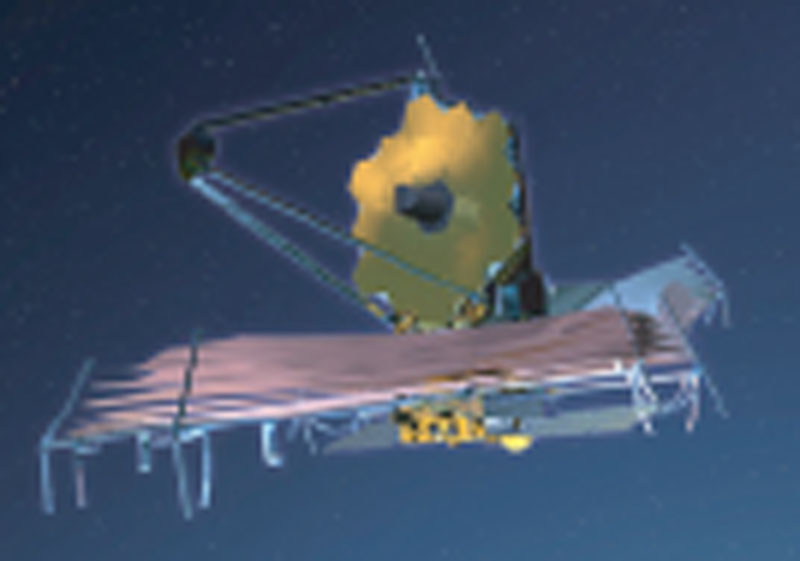 |
Figure 4. A sketch of the current design for the James Webb Space Telescope, the successor to the Hubble Space Telescope to be launched in 2011 (http://www.jwst.nasa.gov/). The current design includes a primary mirror made of beryllium which is 6.5 meter in diameter as well as an instrument sensitivity that spans the full range of infrared wavelengths of 0.6 - 28 µm and will allow detection of the first galaxies in the infant Universe. The telescope will orbit 1.5 million km from Earth at the Lagrange L2 point. |
The next generation of ground-based telescopes will have a diameter of twenty to thirty meter. Together with JWST (that will not be affected by the atmospheric backgound) they will be able to image the first galaxies. Given that these galaxies also created the ionized bubbles around them, the same galaxy locations should correlate with bubbles in the neutral hydrogen (created by their UV emission). Within a decade it would be possible to explore the environmental influence of individual galaxies by using the two sets of instruments in concert [390].
 |
Figure 5. Artist conception of the design for one of the future giant telescopes that could probe the first generation of galaxies from the ground. The Giant Magellan Telescope (GMT) will contain seven mirrors (each 8.4 meter in diameter) and will have the resolving power equivalent to a 24.5 meter (80 foot) primary mirror. For more details see http://www.gmto.org/ |
The dark ingredients of the Universe can only be probed indirectly through a variety of luminous tracers. The distribution and nature of the dark matter are constrained by detailed X-ray and optical observations of galaxies and galaxy clusters. The evolution of the dark energy with cosmic time will be constrained over the coming decade by surveys of Type Ia supernovae, as well as surveys of X-ray clusters, up to a redshift of two.
On large scales (> 10Mpc) the power-spectrum of primordial density
perturbations is already known from the measured microwave background
anisotropies, galaxy surveys, weak lensing, and the
Ly forest. Future programs will refine current knowledge, and will search for
additional trademarks of inflation, such as gravitational waves (through
CMB polarization), small-scale structure (through high-redshift galaxy
surveys and 21cm studies), or the Gaussian statistics of the initial
perturbations.
forest. Future programs will refine current knowledge, and will search for
additional trademarks of inflation, such as gravitational waves (through
CMB polarization), small-scale structure (through high-redshift galaxy
surveys and 21cm studies), or the Gaussian statistics of the initial
perturbations.
The big bang is the only known event where particles with energies
approaching the Planck scale
[( c5
/ G)1/2 ~ 1019 GeV]
interacted. It therefore offers prospects for probing the unification
physics between quantum mechanics and general relativity (to which string
theory is the most-popular candidate). Unfortunately, the exponential
expansion of the Universe during inflation erases memory of earlier cosmic
epochs, such as the Planck time.
c5
/ G)1/2 ~ 1019 GeV]
interacted. It therefore offers prospects for probing the unification
physics between quantum mechanics and general relativity (to which string
theory is the most-popular candidate). Unfortunately, the exponential
expansion of the Universe during inflation erases memory of earlier cosmic
epochs, such as the Planck time.
3.3. Linear Gravitational Growth
Observations of the CMB (e.g., Bennett et al. 1996 [36]) show that the Universe at recombination was extremely uniform, but with spatial fluctuations in the energy density and gravitational potential of roughly one part in 105. Such small fluctuations, generated in the early Universe, grow over time due to gravitational instability, and eventually lead to the formation of galaxies and the large-scale structure observed in the present Universe.
As before, we distinguish between fixed and comoving
coordinates. Using vector notation, the fixed coordinate r
corresponds to a comoving position x = r / a. In a
homogeneous Universe with density
, we describe
the cosmological expansion
in terms of an ideal pressureless fluid of particles each of which is
at fixed x, expanding with the Hubble flow v =
H(t) r where
v = dr / dt. Onto this uniform expansion we
impose small perturbations, given by a relative density perturbation
 |
(9) |
where the mean fluid density is
 , with a
corresponding peculiar velocity
u v -
H r. Then the fluid is described by the
continuity and Euler equations in comoving coordinates
[283,
284]:
, with a
corresponding peculiar velocity
u v -
H r. Then the fluid is described by the
continuity and Euler equations in comoving coordinates
[283,
284]:
 |
(10) (11) |
The potential is
given by the Poisson equation, in terms of the density perturbation:
 |
(12) |
This fluid description is valid for describing the evolution of collisionless cold dark matter particles until different particle streams cross. This "shell-crossing" typically occurs only after perturbations have grown to become non-linear, and at that point the individual particle trajectories must in general be followed. Similarly, baryons can be described as a pressureless fluid as long as their temperature is negligibly small, but non-linear collapse leads to the formation of shocks in the gas.
For small perturbations  << 1, the fluid equations can be linearized and combined to yield
 |
(13) |
This linear equation has in general two independent solutions, only one of which grows with time. Starting with random initial conditions, this "growing mode" comes to dominate the density evolution. Thus, until it becomes non-linear, the density perturbation maintains its shape in comoving coordinates and grows in proportion to a growth factor D(t). The growth factor in the matter-dominated era is given by [283]
 |
(14) |
where we neglect
r when
considering halos forming in the matter-dominated
regime at z << 104. In the Einstein-de Sitter
model (or, at high redshift, in other models as well) the growth factor
is simply proportional to a(t).
The spatial form of the initial density fluctuations can be described in Fourier space, in terms of Fourier components
 |
(15) |
Here we use the comoving wavevector
k, whose magnitude k is the comoving wavenumber which is
equal to 2 divided by the
wavelength. The Fourier description is particularly
simple for fluctuations generated by inflation (e.g., Kolb & Turner 1990
[205]).
Inflation generates perturbations given by a Gaussian
random field, in which different k-modes are statistically
independent,
each with a random phase. The statistical properties of the fluctuations
are determined by the variance of the different k-modes, and the
variance is described in terms of the power spectrum P(k)
as follows:
divided by the
wavelength. The Fourier description is particularly
simple for fluctuations generated by inflation (e.g., Kolb & Turner 1990
[205]).
Inflation generates perturbations given by a Gaussian
random field, in which different k-modes are statistically
independent,
each with a random phase. The statistical properties of the fluctuations
are determined by the variance of the different k-modes, and the
variance is described in terms of the power spectrum P(k)
as follows:
 |
(16) |
where (3)
is the three-dimensional Dirac delta function. The gravitational potential
fluctuations are sourced by the density fluctuations through Poisson's
equation.
In standard models, inflation produces a primordial power-law spectrum
P(k)
kn with n ~ 1. Perturbation growth in the
radiation-dominated and then matter-dominated Universe results in a
modified final power spectrum, characterized by a turnover at a scale
of order the horizon cH-1 at matter-radiation
equality, and a small-scale asymptotic shape of P(k)
kn-4.
The overall amplitude of the power spectrum is not specified by current
models of inflation, and it is usually set by comparing to the observed
CMB temperature fluctuations or to local measures of large-scale
structure.
Since density fluctuations may exist on all scales, in order to determine
the formation of objects of a given size or mass it is useful to consider
the statistical distribution of the smoothed density field. Using a window
function W(r) normalized so that
 d3 r W(r) = 1, the smoothed
density perturbation field,
d3 r
(x)
W(r), itself follows
a Gaussian distribution with zero mean. For the particular choice of a
spherical top-hat, in which W = 1 in a sphere of radius R
and is zero
outside, the smoothed perturbation field measures the fluctuations in the
mass in spheres of radius R. The normalization of the present power
spectrum is often specified by the value of
d3 r W(r) = 1, the smoothed
density perturbation field,
d3 r
(x)
W(r), itself follows
a Gaussian distribution with zero mean. For the particular choice of a
spherical top-hat, in which W = 1 in a sphere of radius R
and is zero
outside, the smoothed perturbation field measures the fluctuations in the
mass in spheres of radius R. The normalization of the present power
spectrum is often specified by the value of
 8
(R = 8
h-1 Mpc). For the top-hat, the smoothed perturbation
field is
denoted r or
m, where the
mass M is related to the
comoving radius R by M = 4
m
R3/3, in terms of the current mean
density of matter m. The variance
< m
>2 is
8
(R = 8
h-1 Mpc). For the top-hat, the smoothed perturbation
field is
denoted r or
m, where the
mass M is related to the
comoving radius R by M = 4
m
R3/3, in terms of the current mean
density of matter m. The variance
< m
>2 is
 |
(17) |
where
j1(x) = (sinx - x cosx) /
x2. The function
(M) plays a crucial
role in estimates of the abundance of collapsed objects, as we describe
later.
Species that decouple from the cosmic plasma (like the dark matter or the baryons) would show fossil evidence for acoustic oscillations in their power spectrum of inhomogeneities due to sound waves in the radiation fluid to which they were coupled at early times. This phenomenon can be understood as follows. Imagine a localized point-like perturbation from inflation at t = 0. The small perturbation in density or pressure will send out a sound wave that will reach the sound horizon cs t at any later time t. The perturbation will therefore correlate with its surroundings up to the sound horizon and all k-modes with wavelengths equal to this scale or its harmonics will be correlated. The scales of the perturbations that grow to become the first collapsed objects at z < 100 cross the horizon in the radiation dominated era after the dark matter decouples from the cosmic plasma. Next we consider the imprint of this decoupling on the smallest-scale structure of the dark matter.
3.4. The Smallest-Scale Power Spectrum of Cold Dark Matter
A broad range of observational data involving the dynamics of galaxies, the growth of large-scale structure, and the dynamics and nucleosynthesis of the Universe as a whole, indicate the existence of dark matter with a mean cosmic mass density that is ~ 5 times larger than the density of the baryonic matter [189, 348]. The data is consistent with a dark matter composed of weakly-interacting, massive particles, that decoupled early and adiabatically cooled to an extremely low temperature by the present time [189]. The Cold Dark Matter (CDM) has not been observed directly as of yet, although laboratory searches for particles from the dark halo of our own Milky-Way galaxy have been able to restrict the allowed parameter space for these particles. Since an alternative more-radical interpretation of the dark matter phenomenology involves a modification of gravity [253], it is of prime importance to find direct fingerprints of the CDM particles. One such fingerprint involves the small-scale structure in the Universe [158], on which we focus in this section.
The most popular candidate for the CDM particle is a Weakly Interacting Massive Particle (WIMP). The lightest supersymmetric particle (LSP) could be a WIMP (for a review see [189]). The CDM particle mass depends on free parameters in the particle physics model but typical values cover a range around M ~ 100 GeV (up to values close to a TeV). In many cases the LSP hypothesis will be tested at the Large Hadron Collider (e.g. [33]) or in direct detection experiments (e.g. [16]).
The properties of the CDM particles affect their response to the small-scale primordial inhomogeneities produced during cosmic inflation. The particle cross-section for scattering off standard model fermions sets the epoch of their thermal and kinematic decoupling from the cosmic plasma (which is significantly later than the time when their abundance freezes-out at a temperature T ~ M). Thermal decoupling is defined as the time when the temperature of the CDM stops following that of the cosmic plasma while kinematic decoupling is defined as the time when the bulk motion of the two species start to differ. For CDM the epochs of thermal and kinetic decoupling coincide. They occur when the time it takes for collisions to change the momentum of the CDM particles equals the Hubble time. The particle mass determines the thermal spread in the speeds of CDM particles, which tends to smooth-out fluctuations on very small scales due to the free-streaming of particles after kinematic decoupling [158, 159]. Viscosity has a similar effect before the CDM fluid decouples from the cosmic radiation fluid [182]. An important effect involves the memory the CDM fluid has of the acoustic oscillations of the cosmic radiation fluid out of which it decoupled. Here we consider the imprint of these acoustic oscillations on the small-scale power spectrum of density fluctuations in the Universe. Analogous imprints of acoustic oscillations of the baryons were identified recently in maps of the CMB [348], and the distribution of nearby galaxies [119]; these signatures appear on much larger scales, since the baryons decouple much later when the scale of the horizon is larger. The discussion in this section follows Loeb & Zaldarriaga (2005) [228].
Formalism
Kinematic decoupling of CDM occurs during the radiation-dominated era. For example, if the CDM is made of neutralinos with a particle mass of ~ 100 GeV, then kinematic decoupling occurs at a cosmic temperature of Td ~ 10 MeV [182, 87]. As long as Td << 100 MeV, we may ignore the imprint of the QCD phase transition (which transformed the cosmic quark-gluon soup into protons and neutrons) on the CDM power spectrum [321]. Over a short period of time during this transition, the pressure does not depend on density and the sound speed of the plasma vanishes, resulting in a significant growth for perturbations with periods shorter than the length of time over which the sound speed vanishes. The transition occurs when the temperature of the cosmic plasma is ~ 100-200 MeV and lasts for a small fraction of the Hubble time. As a result, the induced modifications are on scales smaller than those we are considering here and the imprint of the QCD phase transition is washed-out by the effects we calculate.
At early times the contribution of the dark matter to the energy density is negligible. Only at relatively late times when the cosmic temperature drops to values as low as ~ 1 eV, matter and radiation have comparable energy densities. As a result, the dynamics of the plasma at earlier times is virtually unaffected by the presence of the dark matter particles. In this limit, the dynamics of the radiation determines the gravitational potential and the dark matter just responds to that potential. We will use this simplification to obtain analytic estimates for the behavior of the dark matter transfer function.
The primordial inflationary fluctuations lead to acoustic modes in the radiation fluid during this era. The interaction rate of the particles in the plasma is so high that we can consider the plasma as a perfect fluid down to a comoving scale,
 |
(18) |
where  d
= 0td dt /
a(t) is the conformal time (i.e. the
comoving size of the horizon) at the time of CDM decoupling,
td;
is the scattering cross
section and n is the relevant particle
density. (Throughout this section we set the speed of light and Planck's
constant to unity for brevity.) The damping scale depends on the species
being considered and its contribution to the energy density, and is the
largest for neutrinos which are only coupled through weak interactions. In
that case N ~ (T /
Td
d
= 0td dt /
a(t) is the conformal time (i.e. the
comoving size of the horizon) at the time of CDM decoupling,
td;
is the scattering cross
section and n is the relevant particle
density. (Throughout this section we set the speed of light and Planck's
constant to unity for brevity.) The damping scale depends on the species
being considered and its contribution to the energy density, and is the
largest for neutrinos which are only coupled through weak interactions. In
that case N ~ (T /
Td )3 where Td ~ 1 MeV is the
temperature of neutrino decoupling. At the time of CDM decoupling
N ~ M / Td ~ 104 for the rest
of the plasma, where M is the mass of the
CDM particle. Here we will consider modes of wavelength larger than
)3 where Td ~ 1 MeV is the
temperature of neutrino decoupling. At the time of CDM decoupling
N ~ M / Td ~ 104 for the rest
of the plasma, where M is the mass of the
CDM particle. Here we will consider modes of wavelength larger than
 f, and so
we neglect the effect of radiation diffusion damping
and treat the plasma (without the CDM) as a perfect fluid.
f, and so
we neglect the effect of radiation diffusion damping
and treat the plasma (without the CDM) as a perfect fluid.
The equations of motion for a perfect fluid during the radiation era can be solved analytically. We will use that solution here, following the notation of Dodelson [109]. As usual we Fourier decompose fluctuations and study the behavior of each Fourier component separately. For a mode of comoving wavenumber k in Newtonian gauge, the gravitational potential fluctuations are given by:
 |
(19) |
where  = k
/ 31/2 is the frequency of a mode and
= k
/ 31/2 is the frequency of a mode and
 p is its
primordial amplitude in the limit
p is its
primordial amplitude in the limit
 0. In this section we
use conformal time
=
dt / a(t) with a(t)
t1/2 during
the radiation-dominated era. Expanding the temperature anisotropy in
multipole moments and using the Boltzmann equation to
describe their evolution, the monopole
0. In this section we
use conformal time
=
dt / a(t) with a(t)
t1/2 during
the radiation-dominated era. Expanding the temperature anisotropy in
multipole moments and using the Boltzmann equation to
describe their evolution, the monopole
 0 and
dipole 1 of
the photon distribution can be written in terms of the gravitational
potential as
[109]:
0 and
dipole 1 of
the photon distribution can be written in terms of the gravitational
potential as
[109]:
 |
(20) |
where x
k and a
prime denotes a derivative with respect to x.
The solutions in equations (19) and (20) assume that both the sound speed and the number of relativistic degrees of freedom are constant over time. As a result of the QCD phase transition and of various particles becoming non-relativistic, both of these assumptions are not strictly correct. The vanishing sound speed during the QCD phase transition provides the most dramatic effect, but its imprint is on scales smaller than the ones we consider here because the transition occurs at a significantly higher temperature and only lasts for a fraction of the Hubble time [321].
Before the dark matter decouples kinematically, we will treat it as a fluid which can exchange momentum with the plasma through particle collisions. At early times, the CDM fluid follows the motion of the plasma and is involved in its acoustic oscillations. The continuity and momentum equations for the CDM can be written as:
 |
(21) |
where a dot denotes an -derivative,
c is the dark
matter density perturbation,
c is the
divergence of the dark matter velocity
field and c
denotes the anisotropic stress. In writing these
equations we have followed Ref.
[230].
The term
 c-1
(1 -
c) encodes
the transfer of momentun between the radiation and CDM fluids and
c-1
provides the collisional rate of momentum transfer,
c-1
(1 -
c) encodes
the transfer of momentun between the radiation and CDM fluids and
c-1
provides the collisional rate of momentum transfer,
 |
(22) |
with n being the number density of particles with which the dark
matter is interacting,
(T) the average
cross section for interaction and
M the mass of the dark matter particle. The relevant scattering
partners are the standard model leptons which have thermal
abundances. For detailed expressions of the cross section in the case of
supersymmetric (SUSY) dark matter, see Refs.
[87,
159].
For our purpose, it is sufficient to specify the typical size of the
cross section and its scaling with cosmic time,
 |
(23) |
where the coupling mass
M is
of the order of the weak-interaction
scale (~ 100 GeV) for SUSY dark matter. This equation should be taken
as the definition of
M, as
it encodes all the uncertainties in the
details of the particle physics model into a single parameter. The
temperature dependance of the averaged cross section is a result of the
available phase space. Our results are quite insensitive to the details
other than through the decoupling time. Equating
c-1
/ a to the
Hubble expansion rate gives the temperature of kinematic decoupling:
 |
(24) |
The term k2 cs2
c in
Eq. (21) results from the pressure gradient force and
cs is the dark matter sound speed. In the
tight coupling limit,
c <<
H-1 we find that cs2
 fc
T / M and that the shear term is k2
c
fv
cs2
c
c. Here
fv and fc are constant factors of
order unity. We will find that both these terms make a small difference
on the scales of interest, so their precise value is unimportant.
fc
T / M and that the shear term is k2
c
fv
cs2
c
c. Here
fv and fc are constant factors of
order unity. We will find that both these terms make a small difference
on the scales of interest, so their precise value is unimportant.
By combining both equations in (21) into a single equation
for c we get
 |
(25) |
where xd = k
d and
d
denotes the time of kinematic decoupling
which can be expressed in terms of the decoupling temperature as,
 |
(26) |
with T0 = 2.7K being the present-day CMB temperature and zd being the redshift at kinematic decoupling. We have also introduced the source function,
 |
(27) |
For x << xd, the dark matter sound speed is given by
 |
(28) |
where cs2(xd) is the dark matter sound speed at kinematic decoupling (in units of the speed of light),
 |
(29) |
In writing (28) we have assumed that prior to decoupling the temperature of the dark matter follows that of the plasma. For the viscosity term we have,
 |
(30) |
Free streaming after kinematic decoupling
In the limit of the collision rate being much slower than the Hubble expansion, the CDM is decoupled and the evolution of its perturbations is obtained by solving a Boltzman equation:
 |
(31) |
where f(r, q,
) is the
distribution function which depends on
position, comoving momentum q, and time. The comoving
momentum 3-components are dxi /
d =
qi / a. We use the Boltzman equation to
find the evolution of modes that are well inside the horizon with
x >>
1. In the radiation era, the gravitational potential decays after horizon
crossing (see Eq. 19). In this limit the comoving momentum
remains constant, dqi /
d =0 and
the Boltzman equation becomes,
 |
(32) |
We consider a single Fourier mode and write f as,
 |
(33) |
where f0(q) is the unperturbed distribution,
 |
(34) |
where nCDM and TCDM are the present-day density and temperature of the dark matter.
Our approach is to solve the Boltzman equation with initial conditions
given by the fluid solution at a time
* (which will depend on
k). The simplified Boltzman equation can be easily solved to give
f(q,
) as a function
of the initial conditions f(q,
*),
 |
(35) |
The CDM overdensity
c can then be
expressed in terms of the perturbation in the distribution function as,
 |
(36) |
We can use (35) to obtain the evolution of
c in terms of
its value at
*,
 |
(37) |
where kf-2 = [(Td /
M)]1/2
d.
The exponential term is responsible for the damping of perturbations as
a result of free streaming and
the dispersion of the CDM particles after they decouple from the plasma. The
above expression is only valid during the radiation era. The free streaming
scale is simply given by
dt(v / a)
dta-2 which grows
logarithmically during the radiation era as in equation (37) but
stops growing in the matter era when a
t2/3.
Equation (37) can be used to show that even during the free
streaming epoch,
c satisfies
equation (25) but with a
modified sound speed and viscous term. For x >>
xd one should use,
 |
(38) |
The differences between the above scalings and those during the tight coupling regime are a result of the fact that the dark matter temperature stops following the plasma temperature but rather scales as a-2 after thermal decoupling, which coincides with the kinematic decoupling. We ignore the effects of heat transfer during the fluid stage of the CDM because its temperature is controlled by the much larger heat reservoir of the radiation-dominated plasma at that stage.
To obtain the transfer function we solve the dark matter fluid equation until decoupling and then evolve the overdensity using equation (37) up to the time of matter - radiation equality. In practice, we use the fluid equations up to x* = 10 max(xd, 10) so as to switch into the free streaming solution well after the gravitational potential has decayed. In the fluid equations, we smoothly match the sound speed and viscosity terms at x = xd. As mentioned earlier, because cs(xd) is so small and we are interested in modes that are comparable to the size of the horizon at decoupling, i.e. xd ~ few, both the dark matter sound speed and the associated viscosity play only a minor role, and our simplified treatment is adequate.
In Figure 6 we illustrate the time evolution of
modes during decoupling for a variety of k values. The situation
is clear. Modes that
enter the horizon before kinematic decoupling oscillate with the
radiation fluid. This behavior has two important effects. In the absence of
the coupling, modes receive a "kick" by the source term
S(x) as they
cross the horizon. After that they grow logarithmically. In our case, modes
that entered the horizon before kinematic decoupling follow the plasma
oscillations and thus miss out on both the horizon "kick" and the
beginning of the logarithmic growth. Second, the decoupling from the
radiation fluid is not instantaneous and this acts to further damp the
amplitude of modes with xd >> 1. This effect can
be understood as
follows. Once the oscillation frequency of the mode becomes high compared
to the scattering rate, the coupling to the plasma effectively damps the
mode. In that limit one can replace the forcing term
0' by
its average value, which is close to zero. Thus in this regime, the
scattering is forcing the amplitude of the dark matter oscillations to
zero. After kinematic decoupling the modes again grow logarithmically but
from a very reduced amplitude. The coupling with the plasma induces
both oscillations and damping of modes that entered the horizon before
kinematic decoupling. This damping is different from the free streaming
damping that occurs after kinematic decoupling.
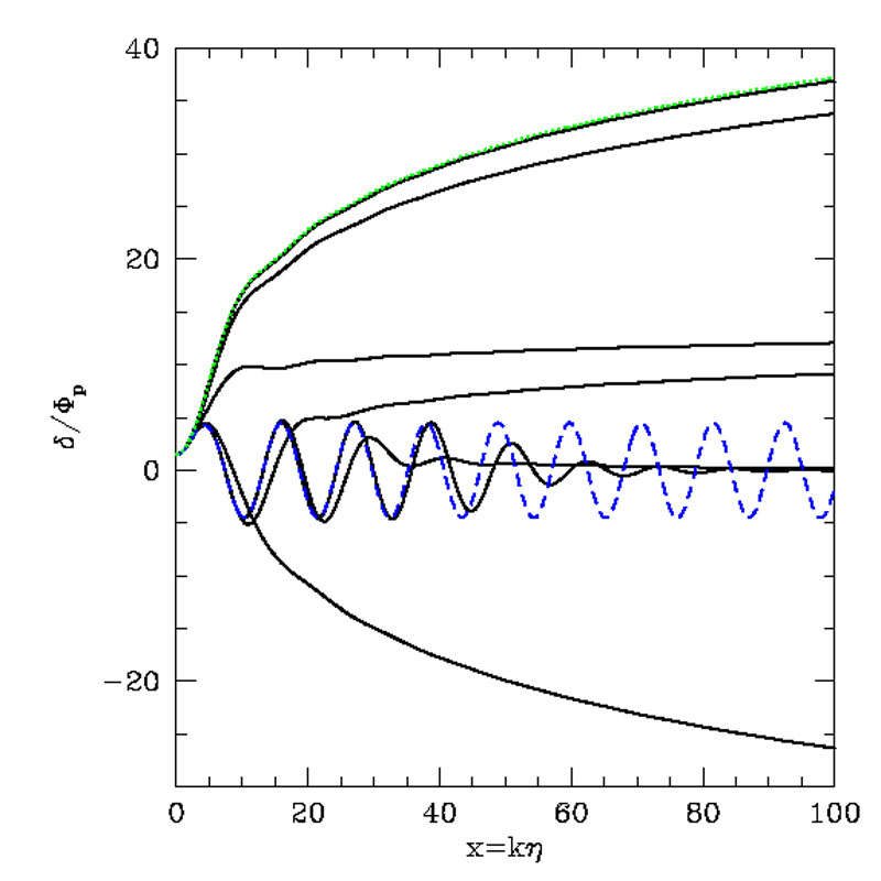 |
Figure 6. The normalized amplitude of CDM
fluctuations |
 |
Figure 7. Transfer function of the CDM density perturbation amplitude (normalized by the primordial amplitude from inflation). We show two cases: (i) Td / M = 10-4 and Td / Teq = 107; (ii) Td / M = 10-5 and Td / Teq = 107. In each case the oscillatory curve is our result and the other curve is the free-streaming only result that was derived previously in the literature [4,7,8]. |
In Figure 7 we show the resulting transfer
function of the
CDM overdensity. The transfer function is defined as the ratio between the
CDM density perturbation amplitude
c when the
effect of the
coupling to the plasma is included and the same quantity in a model where
the CDM is a perfect fluid down to arbitrarily small scales (thus, the
power spectrum is obtained by multiplying the standard result by the square
of the transfer function). This function shows both the oscillations and
the damping signature mentioned above. The peaks occur at multipoles of the
horizon scale at decoupling,
 |
(39) |
This same scale determines the "oscillation" damping. The free streaming damping scale is,
 |
(40) |
where Teq is the temperature at matter radiation equality,
Teq
1 eV. The free streaming scale is parametrically
different from the "oscillation" damping scale. However for our fiducial
choice of parameters for the CDM particle they roughly coincide.
The CDM damping scale is significantly smaller than the scales observed
directly in the Cosmic Microwave Background or through large scale
structure surveys. For example, the ratio of the damping scale to the scale
that entered the horizon at Matter-radiation equality is
d
/ eq
~ Teq / Td ~ 10-7 and to
our present horizon
d
/ 0
~ (Teq T0)1/2 /
Td ~ 10-9. In the
context of inflation, these scales were created 16 and 20 e - folds
apart. Given the large extrapolation, one could certainly imagine that a
change in the spectrum could alter the shape of the power spectrum around
the damping scale. However, for smooth inflaton potentials with small
departures from scale invariance this is not likely to be the case. On
scales much smaller than the horizon at matter radiation equality, the
spectrum of perturbations density before the effects of the damping are
included is approximately,
 |
(41) |
where the first term encodes the shape of the primordial spectrum and the
second the transfer function. Primordial departures from scale invariance
are encoded in the slope n and its running
. The effective slope
at scale k is then,
 |
(42) |
For typical values of (n - 1) ~ 1/60 and
~ 1/602 the
slope is still positive at k ~
d-1, so the cut-off in the power will
come from the effects we calculate rather than from the shape of the
primordial spectrum. However given the large extrapolation in scale, one
should keep in mind the possibility of significant effects resulting from
the mechanisms that generates the density perturbations.
Implications We have found that acoustic oscillations, a relic from the epoch when the dark matter coupled to the cosmic radiation fluid, truncate the CDM power spectrum on a comoving scale larger than effects considered before, such as free-streaming and viscosity [158, 159, 182]. For SUSY dark matter, the minimum mass of dark matter clumps that form in the Universe is therefore increased by more than an order of magnitude to a value of 4
 |
(43) |
where
crit
= (H02 /
8 G) = 9 ×
10-30 g cm-3 is the critical density today, and
m is the
matter density for the concordance cosmological model
[348].
We define the cut-off wavenumber kcut as the point
where the transfer function first drops to a fraction 1 / e of
its value at k
0. This corresponds to kcut
3.3
d-1.
 |
Figure 8. A slice through a numerical
simulation of the first dark matter condensations to form in the
Universe. Colors represent the dark matter density at z =
26. The simulated volume is 60 comoving pc on a side, simulated with 64
million particles each weighing 1.2 × 10⁻¹⁰
M |
Recent numerical simulations [105, 146] of the earliest and smallest objects to have formed in the Universe (see Fig. 3.4), need to be redone for the modified power spectrum that we calculated in this section. Although it is difficult to forecast the effects of the acoustic oscillations through the standard Press-Schechter formalism [291], it is likely that the results of such simulations will be qualitatively the same as before except that the smallest clumps would have a mass larger than before (as given by Eq. 43).
Potentially, there are several observational signatures of the smallest CDM
clumps. As pointed out in the literature
[105,
353],
the smallest CDM clumps could produce
 -rays through
dark-matter annihilation in
their inner density cusps, with a flux in excess of that from nearby dwarf
galaxies. If a substantial fraction of the Milky Way halo is composed of
CDM clumps with a mass ~ 10-4
M
-rays through
dark-matter annihilation in
their inner density cusps, with a flux in excess of that from nearby dwarf
galaxies. If a substantial fraction of the Milky Way halo is composed of
CDM clumps with a mass ~ 10-4
M , the
nearest clump is expected to be at a distance of ~ 4 ×
1017 cm. Given that the characteristic speed of such clumps
is a few hundred km s-1, the
-ray flux
would therefore show temporal variations on the
relatively long timescale of a thousand years. Passage of clumps through
the solar system should also induce fluctuations in the detection rate of
CDM particles in direct search experiments.
Other observational effects have rather limited prospects for
detectability. Because of their relatively low-mass and large size (~
1017 cm), the CDM clumps are too diffuse to produce any
gravitational lensing signatures (including femto-lensing
[161]),
even at cosmological distances.
, the
nearest clump is expected to be at a distance of ~ 4 ×
1017 cm. Given that the characteristic speed of such clumps
is a few hundred km s-1, the
-ray flux
would therefore show temporal variations on the
relatively long timescale of a thousand years. Passage of clumps through
the solar system should also induce fluctuations in the detection rate of
CDM particles in direct search experiments.
Other observational effects have rather limited prospects for
detectability. Because of their relatively low-mass and large size (~
1017 cm), the CDM clumps are too diffuse to produce any
gravitational lensing signatures (including femto-lensing
[161]),
even at cosmological distances.
The smallest CDM clumps should not affect the intergalactic baryons which
have a much larger Jeans mass. However, once objects above ~ 106
M start
to collapse at redshifts z < 30, the baryons would
be able to cool inside of them via molecular hydrogen transitions and the
interior baryonic Jeans mass would drop. The existence of dark matter
clumps could then seed the formation of the first stars inside these
objects
[66].
Early Evolution of Baryonic Perturbations on Large Scales
The baryons are coupled through Thomson scattering to the radiation fluid until they become neutral and decouple. After cosmic recombination, they start to fall into the potential wells of the dark matter and their early evolution was derived by Barkana & Loeb (2005) [29].
On large scales, the dark matter (dm) and the baryons (b) are affected only by their combined gravity and gas pressure can be ignored. The evolution of sub-horizon linear perturbations is described in the matter-dominated regime by two coupled second-order differential equations [284]:
 |
(44) |
where
dm(t)
and b(t)
are the perturbations in the dark matter and baryons, respectively, the
derivatives are with respect to cosmic time t,
H(t) =
 / a is the
Hubble constant with
a = (1 + z)-1, and we assume
that the mean mass density
m(t) is made up of respective mass
fractions fdm and fb = 1 -
fdm. Since these linear
equations contain no spatial gradients, they can be solved spatially for
dm(x,
t) and
b(x,
t) or in Fourier space for
/ a is the
Hubble constant with
a = (1 + z)-1, and we assume
that the mean mass density
m(t) is made up of respective mass
fractions fdm and fb = 1 -
fdm. Since these linear
equations contain no spatial gradients, they can be solved spatially for
dm(x,
t) and
b(x,
t) or in Fourier space for
 dm(k, t) and
b(k, t).
dm(k, t) and
b(k, t).
Defining tot
fb
b +
fdm
dm and
b-
b -
tot , we find
 |
(45) |
Each of these
equations has two independent solutions. The equation for
tot has the
usual growing and decaying solutions, which we denote
D1(t) and D4(t),
respectively, while the
b-
equation has solutions D2(t) and
D3(t); we number the solutions
in order of declining growth rate (or increasing decay rate). We
assume an Einstein-de Sitter, matter-dominated Universe in the
redshift range z = 20 - 150, since the radiation contributes less
than a few percent at z < 150, while the cosmological constant
and the curvature contribute to the energy density less than a few
percent at z > 3. In this regime a
t2/3 and the solutions are
D1(t) = a / ai and
D4(t) = (a /
ai)-3/2 for
tot, and
D2(t) = 1 and D3(t) =
(a / ai)-1/2 for
b-, where we
have normalized each solution to unity at the starting scale factor
ai, which we set at a redshift zi =
150. The observable baryon perturbation can then be written as
 |
(46) |
and similarly for the dark matter perturbation,
 |
(47) |
where Ci = Di for i = 1,4 and
Ci = -(fb /
fdm)Di for
i = 2,3. We may establish the values of
m(k)
by inverting the 4 × 4 matrix A that relates the 4-vector
(1,
2,
3,
4) to the
4-vector that represents the initial conditions
(b,
dm,
b,
dm)
at the initial time.
Next we describe the fluctuations in the sound speed of the cosmic gas
caused by Compton heating of the gas, which is due to scattering of the
residual electrons with the CMB photons. The evolution of the temperature
T of a gas element of density
b
is given by the first law of thermodynamics:
 |
(48) |
where dQ is the heating rate per particle. Before the first galaxies formed,
 |
(49) |
where T is the
Thomson cross-section, xe(t) is the electron
fraction out of the total number density of gas particles, and
is the
CMB energy density at a temperature T. In the
redshift range of interest, we
assume that the photon temperature (T=
T0 / a) is spatially
uniform, since the high sound speed of the photons (i.e., c /
31/2)
suppresses fluctuations on the sub-horizon scales that we consider, and the
horizon-scale ~ 10-5 fluctuations imprinted at cosmic
recombination
are also negligible compared to the smallWe establish the values of
m(k)
by inverting the 4 × 4 matrix A that relates
the 4-vector
(1,
2,
3,
4) to the
4-vector that represents the initial conditions
(b,
dm,
b,
dm)
at the initial time. er-scale fluctuations in the
gas density and temperature. Fluctuations in the residual electron fraction
xe(t) are even smaller. Thus,
 |
(50) |
where t-1
0
(8T c
/ 3 me) = 8.55 × 10⁻¹³ yr-1.
After cosmic recombination, xe(t) changes due
to the slow recombination rate of the residual ions:
 |
(51) |
where
B(T)
is the case-B recombination coefficient of hydrogen,
 H is the mean
number density of hydrogen
at time t, and y = 0.079 is the helium to hydrogen number
density ratio. This yields the evolution of the mean temperature,
d
H is the mean
number density of hydrogen
at time t, and y = 0.079 is the helium to hydrogen number
density ratio. This yields the evolution of the mean temperature,
d  / dt
= - 2 H +
xe(t)
t-1
(T - )
a-4. In prior analyses
[284,
230]
a spatially uniform
speed of sound was assumed for the gas at each redshift. Note that we refer
to p /
as the square
of the sound speed of the fluid,
where p is the
pressure perturbation, although we are analyzing
perturbations driven by gravity rather than sound waves driven by pressure
gradients.
/ dt
= - 2 H +
xe(t)
t-1
(T - )
a-4. In prior analyses
[284,
230]
a spatially uniform
speed of sound was assumed for the gas at each redshift. Note that we refer
to p /
as the square
of the sound speed of the fluid,
where p is the
pressure perturbation, although we are analyzing
perturbations driven by gravity rather than sound waves driven by pressure
gradients.
Instead of assuming a uniform sound speed, we find the first-order perturbation equation,
 |
(52) |
where we defined the fractional temperature perturbation
T. Like
the density perturbation equations, this equation can be solved separately
at each x or at each k. Furthermore, the solution
T (t) is
a linear functional of
b(t)
[for a fixed function xe(t)].
Thus, if we choose an initial time ti then using
Eq. (46) we can write the solution in Fourier space as
 |
(53) |
where DmT(t) is the solution of
Eq. (52) with
T = 0 at
ti and with the
perturbation mode Dm(t) substituted for
b(t),
while D0T(t)
is the solution with no perturbation
b(t)
and with T =
1 at ti. By modifying the CMBFAST code
(http://www.cmbfast.org/), we can
numerically solve Eq. (52) along with the density perturbation
equations for each k down to zi = 150, and then
match the solution to the form of Eq. (53).
Figure 9 shows the time evolution of the various
independent
modes that make up the perturbations of density and temperature, starting
at the time ti corresponding to zi =
150. D2T(t) is identically
zero since D2(t) = 1 is constant, while
D3T(t) and
D4T(t) are
negative. Figure 10 shows the amplitudes of the
various components of the initial perturbations. We consider comoving
wavevectors k in the range 0.01 - 40 Mpc-1, where
the lower limit is set by considering sub-horizon scales at z =
150 for which photon perturbations are negligible compared to
dm and
b, and the
upper limit is set by requiring baryonic pressure to be negligible compared
to gravity.
2 and
3 clearly
show a strong signature of the
large-scale baryonic oscillations, left over from the era of the
photon-baryon fluid before recombination, while
1,
4, and
T
carry only a weak sign of the oscillations. For each quantity, the
plot shows [k3 P(k) /
(2 2)]1/2,
where P(k) is the corresponding power spectrum of
fluctuations.
4 is
already a very small correction
at z = 150 and declines quickly at lower redshift, but the other
three modes all contribute significantly to
b,
and the
T(ti)
term remains significant in
T(t)
even at z < 100. Note that at z = 150 the temperature
perturbation
T has a
different shape with respect to k than the baryon perturbation
b,
showing that
their ratio cannot be described by a scale-independent speed of sound.
 |
Figure 9. Redshift evolution of the amplitudes of the independent modes of the density perturbations (upper panel) and the temperature perturbations (lower panel), starting at redshift 150 (from Barkana & Loeb 2005 [29]). We show m = 1 (solid curves), m = 2 (short-dashed curves), m = 3 (long-dashed curves), m = 4 (dotted curves), and m = 0 (dot-dashed curve). Note that the lower panel shows one plus the mode amplitude. |
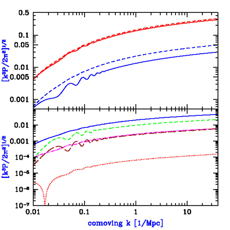 |
Figure 10. Power spectra and initial
perturbation amplitudes versus wavenumber (from
[29]).
The upper panel shows
|
The power spectra of the various perturbation modes and of
T(ti) depend on the
initial power spectrum of density fluctuations from inflation and on the
values of the fundamental cosmological parameters
(dm,
b,
,
and h). If these independent power spectra can
be measured through 21cm fluctuations, this will probe the basic
cosmological parameters through multiple combinations, allowing
consistency checks that can be used to verify the adiabatic nature and
the expected history of the perturbations.
Figure 11 illustrates the relative sensitivity of
[P(k)]1/2 to variations in
dm
h2,
b
h2, and h, for the quantities
1,
2,
3, and
T(ti). Not shown is
4,
which although it is more sensitive (changing by order unity due to
10% variations in the parameters), its magnitude always remains
much smaller than the other modes, making it much harder to
detect. Note that although the angular scale of the baryon
oscillations constrains also the history of dark energy through the
angular diameter distance, we have focused here on other cosmological
parameters, since the contribution of dark energy relative to matter
becomes negligible at high redshift.
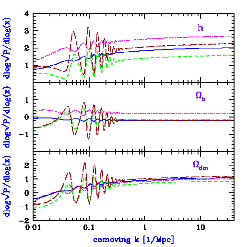 |
Figure 11. Relative sensitivity of
perturbation amplitudes at z = 150 to cosmological parameters (from
[29]).
For variations in a parameter
x, we show d log [P(k)]1/2
/ d log(x). We consider variations
in |
Cosmological Jeans Mass
The Jeans length
J was
originally defined (Jeans 1928
[187])
in Newtonian
gravity as the critical wavelength that separates oscillatory and
exponentially-growing density perturbations in an infinite, uniform, and
stationary distribution of gas. On scales
 smaller than
J,
the sound crossing time, /
cs is shorter than the gravitational
free-fall time, (G
)-1/2,
allowing the build-up of a pressure force
that counteracts gravity. On larger scales, the pressure gradient force is
too slow to react to a build-up of the attractive gravitational force. The
Jeans mass is defined as the mass within a sphere of radius
J / 2,
MJ = (4 / 3)
(J /
2)3. In a perturbation with a mass greater than
MJ, the self-gravity cannot be supported by the
pressure
gradient, and so the gas is unstable to gravitational collapse. The
Newtonian derivation of the Jeans instability suffers from a conceptual
inconsistency, as the unperturbed gravitational force of the uniform
background must induce bulk motions (compare to Binney & Tremaine 1987
[43]).
However, this inconsistency is remedied when the analysis is
done in an expanding Universe.
smaller than
J,
the sound crossing time, /
cs is shorter than the gravitational
free-fall time, (G
)-1/2,
allowing the build-up of a pressure force
that counteracts gravity. On larger scales, the pressure gradient force is
too slow to react to a build-up of the attractive gravitational force. The
Jeans mass is defined as the mass within a sphere of radius
J / 2,
MJ = (4 / 3)
(J /
2)3. In a perturbation with a mass greater than
MJ, the self-gravity cannot be supported by the
pressure
gradient, and so the gas is unstable to gravitational collapse. The
Newtonian derivation of the Jeans instability suffers from a conceptual
inconsistency, as the unperturbed gravitational force of the uniform
background must induce bulk motions (compare to Binney & Tremaine 1987
[43]).
However, this inconsistency is remedied when the analysis is
done in an expanding Universe.
The perturbative derivation of the Jeans instability criterion can be
carried out in a cosmological setting by considering a sinusoidal
perturbation superposed on a uniformly expanding background. Here, as
in the Newtonian limit, there is a critical wavelength
J that
separates oscillatory and growing modes. Although the expansion of
the background slows down the exponential growth of the amplitude to a
power-law growth, the fundamental concept of a minimum mass that can
collapse at any given time remains the same (see, e.g. Kolb & Turner
1990
[205];
Peebles 1993
[284]).
We consider a mixture of dark matter and baryons with density parameters
dmz =
dm
/ c
and
bz =
b /
c,
where
dm is the average dark matter density,
b is the average baryonic density,
c is
the critical density, and
dmz +
bz =
mz is given by
equation(83). We also assume spatial fluctuations in the gas and
dark matter densities with the form of a single spherical Fourier mode
on a scale much smaller than the horizon,
 |
(54) (55) |
where dm(t) and
b(t) are the
background densities of the dark matter and baryons,
dm(t)
and
b(t)
are the dark matter and baryon overdensity amplitudes, r is the
comoving radial coordinate, and k
is the comoving perturbation wavenumber. We adopt an ideal gas
equation-of-state for the baryons with a specific heat ratio
=
5/3. Initially, at time t = ti, the gas
temperature is uniform Tb(r,
ti) = Ti, and the
perturbation amplitudes are small
dm,i,
b,i <<
1. We define the region inside the first zero of
sin(kr) / (kr), namely 0 < kr <
, as the collapsing "object".
The evolution of the temperature of the baryons
Tb(r, t) in
the linear regime is determined by the coupling of their free
electrons to the CMB through Compton
scattering, and by the adiabatic expansion of the gas. Hence,
Tb(r, t) is generally somewhere between
the CMB temperature,
T
(1 +
z)-1 and the adiabatically-scaled
temperature Tad
(1 +
z)-2. In the limit of tight
coupling to T, the gas temperature remains uniform. On the
other hand, in the adiabatic limit, the temperature develops a
gradient according to the relation
 |
(56) |
The evolution of a cold dark matter overdensity,
dm(t),
in the linear regime is described by the equation (44),
 |
(57) |
whereas the evolution of the overdensity of the baryons,
b(t),
with the inclusion of their pressure force is described by
(see Section 9.3.2 of
[205]),
 |
(58) |
Here, H(t) =
/ a is the
Hubble parameter at a cosmological time
t, and µ = 1.22 is the mean molecular weight of the
neutral primordial gas in atomic units. The parameter
 distinguishes
between the two limits for the evolution of the gas temperature. In
the adiabatic limit
= 1, and
when the baryon temperature is
uniform and locked to the background radiation,
= 0. The last
term on the right hand side (in square brackets) takes into account
the extra pressure gradient force in
distinguishes
between the two limits for the evolution of the gas temperature. In
the adiabatic limit
= 1, and
when the baryon temperature is
uniform and locked to the background radiation,
= 0. The last
term on the right hand side (in square brackets) takes into account
the extra pressure gradient force in
 (b
T) = (T
b
+ b
T), arising from
the temperature
gradient which develops in the adiabatic limit. The Jeans wavelength
J =
2 / kJ is
obtained by setting the right-hand side of
equation (58) to zero, and solving for the critical wavenumber
kJ. As can be seen from equation (58), the critical
wavelength
J (and
therefore the mass MJ) is in general
time-dependent. We infer from equation (58) that as time
proceeds, perturbations with increasingly smaller initial wavelengths
stop oscillating and start to grow.
(b
T) = (T
b
+ b
T), arising from
the temperature
gradient which develops in the adiabatic limit. The Jeans wavelength
J =
2 / kJ is
obtained by setting the right-hand side of
equation (58) to zero, and solving for the critical wavenumber
kJ. As can be seen from equation (58), the critical
wavelength
J (and
therefore the mass MJ) is in general
time-dependent. We infer from equation (58) that as time
proceeds, perturbations with increasingly smaller initial wavelengths
stop oscillating and start to grow.
To estimate the Jeans wavelength, we equate the right-hand-side of
equation (58) to zero. We further approximate
b ~
dm, and
consider sufficiently high redshifts at
which the Universe is matter dominated and flat,
(1 + z) >> max[(1 -
m -
) /
m,
( /
m)1/3]. In this regime,
b
<< m
1, H
2 / (3t), and
a = (1 + z)-1
(3H0
(m)1/2 / 2)2/3
t2/3, where
m
= dm
+ b is
the total matter
density parameter. Following cosmological recombination at z
103, the residual ionization of the cosmic gas keeps its
temperature locked to the CMB temperature (via Compton scattering) down
to a redshift of
[284]
 |
(59) |
In the redshift range between recombination and zt,
= 0 and
 |
(60) |
so that the Jeans mass is therefore redshift independent and obtains the value (for the total mass of baryons and dark matter)
 |
(61) |
Based on the similarity of MJ to the mass of a globular cluster, Peebles & Dicke (1968) [281] suggested that globular clusters form as the first generation of baryonic objects shortly after cosmological recombination. Peebles & Dicke assumed a baryonic Universe, with a nonlinear fluctuation amplitude on small scales at z ~ 103, a model which has by now been ruled out. The lack of a dominant mass of dark matter inside globular clusters makes it unlikely that they formed through direct cosmological collapse, and more likely that they resulted from fragmentation during the process of galaxy formation.
 |
Figure 12. Thermal history of the baryons,
left over from the big bang, before the first galaxies formed. The
residual fraction of free electrons couple the gas temperture
Tgas
to the cosmic microwave background temperature
[T |
At z < zt, the gas temperature declines
adiabatically as [(1 + z) / ( 1 +
zt)]2 (i.e.,
= 1) and
the total Jeans mass obtains the value,
 |
(62) |
It is not clear how the value of the Jeans mass derived above relates
to the mass of collapsed, bound objects. The above analysis is
perturbative (Eqs. 57 and 58 are valid only as long as
b and
dm are much
smaller than unity),
and thus can only describe the initial phase of the collapse. As
b and
dm grow and
become larger than
unity, the density profiles start to evolve and dark matter shells may
cross baryonic shells
[167]
due to their
different dynamics. Hence the amount of mass enclosed within a given
baryonic shell may increase with time, until eventually the dark
matter pulls the baryons with it and causes their collapse even
for objects below the Jeans mass.
Even within linear theory, the Jeans mass is related only to the evolution
of perturbations at a given time. When the Jeans mass itself varies with
time, the overall suppression of the growth of perturbations depends on a
time-weighted Jeans mass. Gnedin & Hui (1998)
[150]
showed that the correct time-weighted mass is the filtering mass
Mf = (4 /3)
(2 a /
kf)3, in terms of the comoving wavenumber
kf
associated with the "filtering scale" (note the change in convention from
/ kJ to
2 / kf). The
wavenumber kf is related to the Jeans
wavenumber kJ by
 |
(63) |
where D(t) is the linear
growth factor. At high redshift (where
mz
1), this
relation simplifies to
[153]
 |
(64) |
Then the relationship between the linear overdensity of the
dark matter dm
and the linear overdensity of the baryons
b,
in the limit of small k, can be written as
[150]
 |
(65) |
Linear theory specifies whether an initial perturbation, characterized
by the parameters k,
dm,i,
b,i and
ti, begins to grow. To determine the minimum mass of
nonlinear baryonic objects resulting from the shell-crossing and
virialization of the dark matter, we must use a different model which
examines the response of the gas to the gravitational potential of a
virialized dark matter halo.
3.6. Formation of Nonlinear Objects
Let us consider a spherically symmetric density or velocity perturbation of
the smooth cosmological background, and examine the dynamics of a test
particle at a radius r relative to the center of symmetry. Birkhoff's
(1923)
[44]
theorem implies that we may ignore the mass outside this radius in
computing the motion of our particle. We further find that the
relativistic equations of motion describing the system reduce to the usual
Friedmann equation for the evolution of the scale factor of a homogeneous
Universe, but with a density parameter
that now takes
account of
the additional mass or peculiar velocity. In particular, despite the
arbitrary density and velocity profiles given to the perturbation, only the
total mass interior to the particle's radius and the peculiar velocity at
the particle's radius contribute to the effective value of
. We
thus find a solution to the particle's motion which describes its departure
from the background Hubble flow and its subsequent collapse or expansion.
This solution holds until our particle crosses paths with one from a
different radius, which happens rather late for most initial profiles.
As with the Friedmann equation for a smooth Universe, it is possible to reinterpret the problem into a Newtonian form. Here we work in an inertial (i.e. non-comoving) coordinate system and consider the force on the particle as that resulting from a point mass at the origin (ignoring the possible presence of a vacuum energy density):
 |
(66) |
where G is Newton's constant, r is the distance of the particle from the center of the spherical perturbation, and M is the total mass within that radius. As long as the radial shells do not cross each other, the mass M is constant in time. The initial density profile determines M, while the initial velocity profile determines dr / dt at the initial time. As is well-known, there are three branches of solutions: one in which the particle turns around and collapses, another in which it reaches an infinite radius with some asymptotically positive velocity, and a third intermediate case in which it reachs an infinite radius but with a velocity that approaches zero. These cases may be written as [164]:
 |
(67) |
 |
(68) |
 |
(69) |
where A3 = GMB2 applies in
all cases. All three solutions have
r3 = 9GMt2 / 2 as t
goes to zero, which matches the linear theory
expectation that the perturbation amplitude get smaller as one goes back
in time. In the closed case, the shell turns around at time
B and
radius 2A and collapses to zero radius at time
2 B.
We are now faced with the problem of relating the spherical collapse
parameters A, B, and M to the linear theory density
perturbation
[283].
We do this by returning to the equation of motion. Consider that at an
early epoch (i.e. scale factor ai << 1),
we are given a spherical patch of uniform overdensity
i (the
so-called `top-hat' perturbation). If
is essentially unity at
this time and if the perturbation is pure growing mode, then the initial
velocity is radially inward with magnitude
i
H(ti)r / 3, where
H(ti) is the Hubble constant at the initial
time and r is the radius
from the center of the sphere. This can be easily seen from the continuity
equation in spherical coordinates. The equation of motion (in noncomoving
coordinates) for a particle beginning at radius ri is
simply
 |
(70) |
where M = (4 / 3)
ri3
i (1
+ i) and
i
is the background density of the Universe at time
ti. We next define
the dimensionless radius x = rai /
ri and rewrite equation (70) as
 |
(71) |
Our initial conditions for the integration of this orbit are
 |
(72) |
 |
(73) |
where H(t1) =
H0[m / a3(t1) +
(1 - m)]1/2 is the Hubble
parameter for a flat Universe at a a cosmic time
t1. Integrating equation (71) yields
 |
(74) |
where K is a constant of integration. Evaluating this at the initial
time and dropping terms of O(ai) (but
i ~
ai, so we keep ratios of order unity), we find
 |
(75) |
If K is sufficiently negative, the particle will turn-around and the sphere will collapse at a time
 |
(76) |
where amax is the value of a which sets the denominator of the integral to zero.
For the case of
= 0, we can determine the spherical collapse
parameters A and B. K > 0 (K < 0)
produces an open (closed) model.
Comparing coefficients in the energy equations [eq. (74) and the
integration of (66)], one finds
 |
(77) |
 |
(78) |
where k =
1 - m.
In particular, in an
= 1
Universe, where 1 + z = (3H0 t /
2)-2/3, we find that a shell collapses
at redshift 1 + zc =
0.5929i /
ai, or in other words a shell
collapsing at redshift zc had a linear overdensity
extrapolated to the present day of
0 = 1.686(1 +
zc).
While this derivation has been for spheres of constant density, we may
treat a general spherical density profile
i(r)
up until shell crossing
[164].
A particular radial shell evolves according to the mass interior to it;
therefore, we define the average overdensity

 |
(79) |
so that we may use
in place of
i in the
above formulae. If
is not monotonically decreasing with R, then the spherical top-hat
evolution of two different radii will predict that they cross each other
at some late time; this is known as shell crossing and signals the
breakdown of the solution. Even well-behaved
profiles will produce shell crossing if
shells are allowed to collapse to r = 0 and then reexpand, since
these
expanding shells will cross infalling shells. In such a case, first-time
infalling shells will never be affected prior to their turn-around; the
more complicated behavior after turn-around is a manifestation of
virialization. While the end state for general initial conditions cannot
be predicted, various results are known for a self-similar collapse, in
which
(r) is a
power-law
[132,
40],
as well as for the case of secondary infall models
[156,
165,
181].
The small density fluctuations evidenced in the CMB grow over time as
described in the previous subsection, until the perturbation
becomes of order unity, and the full non-linear gravitational problem
must be considered. The dynamical collapse of a dark matter halo can
be solved analytically only in cases of particular symmetry. If we
consider a region which is much smaller than the horizon
cH-1,
then the formation of a halo can be formulated as a problem in
Newtonian gravity, in some cases with minor corrections coming from
General Relativity. The simplest case is that of spherical symmetry,
with an initial (t = ti <<
t0) top-hat of uniform overdensity
i inside a
sphere of radius R. Although this model is
restricted in its direct applicability, the results of spherical
collapse have turned out to be surprisingly useful in understanding
the properties and distribution of halos in models based on cold dark
matter.
The collapse of a spherical top-hat perturbation is described by the Newtonian equation (with a correction for the cosmological constant)
 |
(80) |
where r is the
radius in a fixed (not comoving) coordinate frame, H0
is the present-day Hubble constant, M is the total mass enclosed
within radius r, and the
initial velocity field is given by the Hubble flow dr / dt
= H(t) r. The
enclosed grows
initially as L =
i
D(t) / D(ti), in
accordance with linear theory, but eventually
grows above
L. If the
mass shell at radius r is bound (i.e., if its total
Newtonian energy is negative) then it reaches a radius of maximum expansion
and subsequently collapses. As demonstrated in the previous section, at the
moment when the top-hat collapses to a point, the overdensity predicted by
linear theory is
L = 1.686 in
the Einstein-de Sitter model, with only a weak dependence on
m and
. Thus a tophat collapses at
redshift z if its linear overdensity extrapolated to the present day
(also termed the critical density of collapse) is
 |
(81) |
where we set D(z = 0) = 1.
Even a slight violation of the exact symmetry of the initial perturbation
can prevent the tophat from collapsing to a point. Instead, the halo
reaches a state of virial equilibrium by violent relaxation (phase
mixing). Using the virial theorem U = -2K to relate the
potential energy U to the kinetic energy K in the final
state (implying that the virial
radius is half the turnaround radius - where the kinetic energy vanishes),
the final overdensity relative to the critical density at the collapse
redshift is
 c =
182
c =
182
 178 in the Einstein-de
Sitter model, modified in a Universe with
m +
= 1
to the fitting formula (Bryan & Norman 1998
[71])
178 in the Einstein-de
Sitter model, modified in a Universe with
m +
= 1
to the fitting formula (Bryan & Norman 1998
[71])
 |
(82) |
where d
mz-1 is evaluated at the collapse
redshift, so that
 |
(83) |
A halo of mass M collapsing at redshift z thus has a virial radius
 |
(84) |
and a corresponding circular velocity,
 |
(85) |
In these expressions we have assumed a present Hubble constant written in the form H0 = 100 h km s-1Mpc-1. We may also define a virial temperature
 |
(86) |
where µ is the mean molecular weight and mp is the proton mass. Note that the value of µ depends on the ionization fraction of the gas; for a fully ionized primordial gas µ = 0.59, while a gas with ionized hydrogen but only singly-ionized helium has µ = 0.61. The binding energy of the halo is approximately 5
 |
(87) |
Note that the binding energy of the baryons
is smaller by a factor equal to the baryon fraction
b /
m.
Although spherical collapse captures some of the physics governing the formation of halos, structure formation in cold dark matter models procedes hierarchically. At early times, most of the dark matter is in low-mass halos, and these halos continuously accrete and merge to form high-mass halos. Numerical simulations of hierarchical halo formation indicate a roughly universal spherically-averaged density profile for the resulting halos (Navarro, Frenk, & White 1997, hereafter NFW [266]), though with considerable scatter among different halos (e.g., [72]). The NFW profile has the form
 |
(88) |
where x = r / rvir, and the
characteristic density
c is related
to the concentration parameter cN by
 |
(89) |
The concentration parameter itself depends on the halo mass M, at a given redshift z [377].
More recent N-body simulations indicate deviations from the original NFW profile; for details and refined fitting formula see [268].
1 http://www.eso.org/projects/owl/ Back.
2 http://celt.ucolick.org/ Back.
4 Our definition of the cut-off mass
follows the convention of the
Jeans mass, which is defined as the mass enclosed within a sphere of radius
J/2 where
J
2 / kJ is the
Jeans wavelength
[168].
Back.
5 The coefficient of 1/2 in
equation (87) would be exact for a singular isothermal sphere,
(r)
1/r2.
Back.