


4.1. The Abundance of Dark Matter Halos
In addition to characterizing the properties of individual halos, a critical prediction of any theory of structure formation is the abundance of halos, i.e. the number density of halos as a function of mass, at any redshift. This prediction is an important step toward inferring the abundances of galaxies and galaxy clusters. While the number density of halos can be measured for particular cosmologies in numerical simulations, an analytic model helps us gain physical understanding and can be used to explore the dependence of abundances on all the cosmological parameters.
A simple analytic model which successfully matches most of the numerical
simulations was developed by Press & Schechter (1974)
[291]. The model is based
on the ideas of a Gaussian random field of density perturbations, linear
gravitational growth, and spherical collapse. To determine the abundance of
halos at a redshift z, we use
 m, the
density field smoothed on a mass scale M, as defined in
Section 3.3. Since
m is
distributed as a Gaussian variable with zero mean and standard deviation
m, the
density field smoothed on a mass scale M, as defined in
Section 3.3. Since
m is
distributed as a Gaussian variable with zero mean and standard deviation
 (M) [which
depends only on the present linear power spectrum, see
equation (17)], the probability that
m is greater than
some equals
(M) [which
depends only on the present linear power spectrum, see
equation (17)], the probability that
m is greater than
some equals
 |
(90) |
The fundamental ansatz is to
identify this probability with the fraction of dark matter particles which
are part of collapsed halos of mass greater than M, at redshift
z. There are two additional ingredients: First, the value used for
is
crit(z)
given in equation (81), which is the critical density of collapse found
for a spherical top-hat (extrapolated to the present since
(M) is calculated
using the present power spectrum); and second, the fraction of dark
matter in halos above M is multiplied by an additional factor of
2 in order to ensure that every particle ends up as part of some halo
with M > 0. Thus, the final formula for the mass fraction in
halos above M at redshift z is
 |
(91) |
This ad-hoc factor of 2 is necessary, since otherwise only positive
fluctuations of
m would be
included. Bond et al. (1991)
[52]
found an alternate derivation of this correction factor, using a
different ansatz. In their derivation, the factor of 2 has a more
satisfactory origin, namely the so-called "cloud-in-cloud" problem:
For a given mass M, even if
m is smaller
than
crit(z),
it is possible that the corresponding region lies inside a
region of some larger mass ML > M, with
ML
> crit(z). In this case the original region
should be counted as belonging to a halo of mass
ML. Thus, the fraction of particles
which are part of collapsed halos of mass greater than M is larger
than the expression given in equation (90). Bond et al. showed
that, under certain assumptions, the additional contribution results
precisely in a factor of 2 correction.
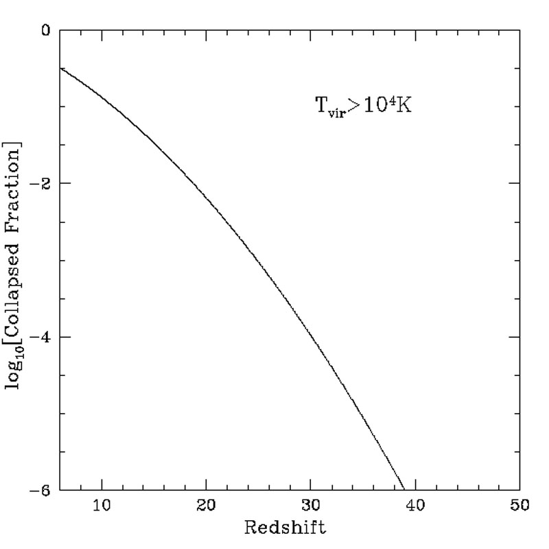 |
Figure 13. Fraction of baryons that assembled into dark matter halos with a virial temperature of Tvir > 104K as a function of redshift. These baryons are above the temperature threshold for gas cooling and fragmentation via atomic transitions. After reionization the temperature barrier for star formation in galaxies is raised because the photo-ionized intergalactic medium is already heated to ~ 104K and it can condense only into halos with Tvir > 105K. |
Differentiating the fraction of dark matter in halos above M yields the mass distribution. Letting dn be the comoving number density of halos of mass between M and M + dM, we have
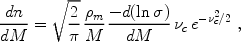 |
(92) |
where  c =
crit(z)
/ (M) is the
number of standard deviations which the critical
collapse overdensity represents on mass scale M. Thus, the abundance
of halos depends on the two functions
(M) and
crit (z),
each of which depends on the energy content of the
Universe and the values of the other cosmological parameters. Since
recent observations confine the standard set of parameters to a
relatively narrow range, we illustrate the abundance of halos and
other results for a single set of parameters:
c =
crit(z)
/ (M) is the
number of standard deviations which the critical
collapse overdensity represents on mass scale M. Thus, the abundance
of halos depends on the two functions
(M) and
crit (z),
each of which depends on the energy content of the
Universe and the values of the other cosmological parameters. Since
recent observations confine the standard set of parameters to a
relatively narrow range, we illustrate the abundance of halos and
other results for a single set of parameters:
 m = 0.3,
 = 0.7,
b =
0.045, 8 =
0.9, a primordial power spectrum index n = 1 and a Hubble
constant h = 0.7.
= 0.7,
b =
0.045, 8 =
0.9, a primordial power spectrum index n = 1 and a Hubble
constant h = 0.7.
Figure 14 shows
(M) and
crit(z),
with the input power spectrum computed from Eisenstein & Hu (1999)
[118].
The solid line is
(M) for the cold
dark matter model with the parameters specified above. The horizontal
dotted lines show the value of
crit(z)
at z = 0, 2, 5, 10, 20 and 30, as indicated
in the figure. From the intersection of these horizontal lines with
the solid line we infer, e.g., that at z = 5 a
1- fluctuation
on a mass scale of 2 × 10⁷
M will
collapse. On the other hand, at z = 5 collapsing halos require a
2- fluctuation on a
mass scale of 3 × 10¹⁰
M, since
(M) on this
mass scale equals about half of
crit(z
= 5). Since at each redshift a fixed fraction (31.7%) of the total dark
matter mass lies in halos above the
1- mass,
Figure 14 shows
that most of the mass is in small halos at high redshift, but it
continuously shifts toward higher characteristic halo masses at lower
redshift. Note also that
(M) flattens at
low masses because of the changing shape of the power spectrum. Since
will
collapse. On the other hand, at z = 5 collapsing halos require a
2- fluctuation on a
mass scale of 3 × 10¹⁰
M, since
(M) on this
mass scale equals about half of
crit(z
= 5). Since at each redshift a fixed fraction (31.7%) of the total dark
matter mass lies in halos above the
1- mass,
Figure 14 shows
that most of the mass is in small halos at high redshift, but it
continuously shifts toward higher characteristic halo masses at lower
redshift. Note also that
(M) flattens at
low masses because of the changing shape of the power spectrum. Since

 as M
0, in the cold dark matter model all the
dark matter is tied up in halos at all redshifts, if sufficiently
low-mass halos are considered.
as M
0, in the cold dark matter model all the
dark matter is tied up in halos at all redshifts, if sufficiently
low-mass halos are considered.
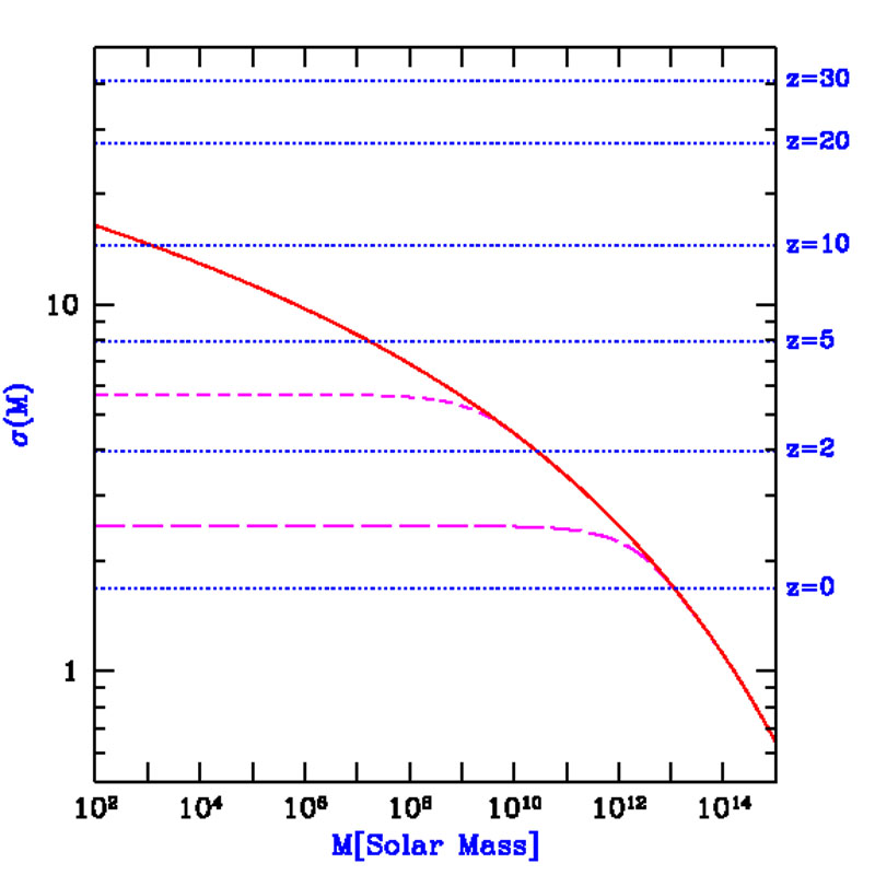 |
Figure 14. Mass fluctuations and collapse
thresholds in cold dark matter models. The horizontal dotted lines show
the value of the extrapolated collapse overdensity
|
Also shown in Figure 14 is the effect of
cutting off the power spectrum on small scales. The short-dashed curve
corresponds to the case where the power spectrum is set to zero above a
comoving wavenumber k = 10 Mpc-1, which
corresponds to a mass M = 1.7 × 10⁸
M. The
long-dashed curve corresponds to a
more radical cutoff above k = 1 Mpc-1, or below
M = 1.7 × 10¹¹
M. A
cutoff severely reduces the
abundance of low-mass halos, and the finite value of
(M = 0)
implies that at all redshifts some fraction of the dark matter does
not fall into halos. At high redshifts where
crit(z)
>>
(M = 0), all
halos are rare and only a small fraction of the dark
matter lies in halos. In particular, this can affect the abundance of
halos at the time of reionization, and thus the observed limits on
reionization constrain scenarios which include a small-scale cutoff in
the power spectrum
[21].
In figures 15 - 18
we show explicitly the properties of collapsing halos which represent
1-,
2-, and
3-
fluctuations (corresponding in all cases to the curves in order from bottom
to top), as a function of redshift. No cutoff is applied to the power
spectrum. Figure 15 shows the halo mass,
Figure 16 the
virial radius, Figure 17 the virial temperature
(with µ in equation (86) set equal to 0.6, although low
temperature halos contain neutral gas) as well as circular velocity, and
Figure 18
shows the total binding energy of these halos. In
figures 15 and
17, the dotted curves indicate the minimum
virial temperature
required for efficient cooling with primordial atomic species only (upper
curve) or with the addition of molecular hydrogen (lower curve).
Figure 18 shows the binding energy of dark
matter halos. The binding energy of the baryons is a factor ~
b /
m ~ 15%
smaller, if they follow the dark matter. Except for this constant factor,
the figure shows the minimum amount of energy that needs to be deposited
into the gas in order to unbind it from the potential well of the dark
matter. For example, the hydrodynamic energy released by a single
supernovae, ~ 1051 erg, is sufficient to unbind the gas in
all 1- halos at z
> 5 and in all 2-
halos at z > 12.
 |
Figure 15. Characteristic properties of
collapsing halos: Halo mass.
The solid curves show the mass of collapsing halos which correspond to
1- |
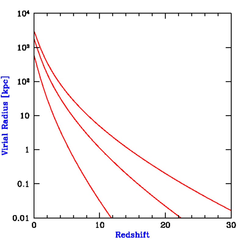 |
Figure 16. Characteristic properties of
collapsing halos: Halo virial
radius. The curves show the virial radius of collapsing halos which
correspond to
1- |
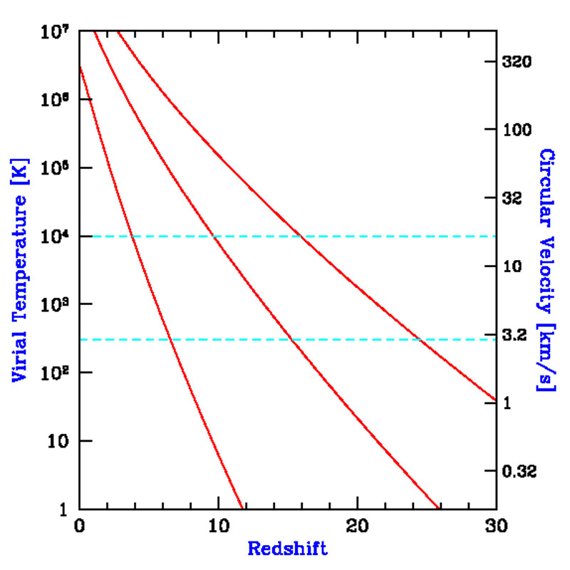 |
Figure 17. Characteristic properties of
collapsing halos: Halo virial
temperature and circular velocity. The solid curves show the virial
temperature (or, equivalently, the circular velocity) of collapsing
halos which correspond to
1- |
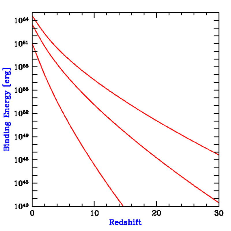 |
Figure 18. Characteristic properties of
collapsing halos: Halo binding
energy. The curves show the total binding energy of collapsing halos
which correspond to
1- |
At z = 5, the halo masses which correspond to
1-,
2-,
and 3- fluctuations are
1.8 × 10⁷
M, 3.0
× 1010
M, and
7.0 × 10¹¹
M,
respectively. The
corresponding virial temperatures are 2.0 × 10³ K, 2.8
× 105 K, and 2.3 × 10⁶ K. The equivalent
circular velocities are 7.5 km s-1, 88 km s-1, and
250 km s-1. At z = 10, the
1-,
2-, and
3-
fluctuations correspond to halo masses of 1.3 × 10³
M,
5.7 × 10⁷
M, and
4.8 × 10⁹
M,
respectively. The corresponding virial temperatures are 6.2 K, 7.9
× 103 K, and 1.5 × 10⁵ K. The equivalent
circular velocities are 0.41 km s-1, 15 km s-1, and 65
km s-1. Atomic cooling is efficient at Tvir
> 104 K, or a circular velocity Vc >
17 km s-1. This corresponds to a
1.2- fluctuation and a
halo mass of 2.1 × 10⁸
M at
z = 5, and a
2.1- fluctuation and
a halo mass of 8.3 × 10⁷
M at
z = 10. Molecular hydrogen
provides efficient cooling down to Tvir ~ 300 K, or a
circular velocity Vc ~ 2.9 km s-1. This
corresponds to a 0.81-
fluctuation and a halo mass of 1.1 × 10⁶
M at
z = 5, and a 1.4-
fluctuation and a halo mass of 4.3 × 10⁵
M at
z = 10.
In Figure 19 we show the halo mass function dn / dln(M) at several different redshifts: z = 0 (solid curve), z = 5 (dotted curve), z = 10 (short-dashed curve), z = 20 (long-dashed curve), and z = 30 (dot-dashed curve). Note that the mass function does not decrease monotonically with redshift at all masses. At the lowest masses, the abundance of halos is higher at z > 0 than at z = 0.
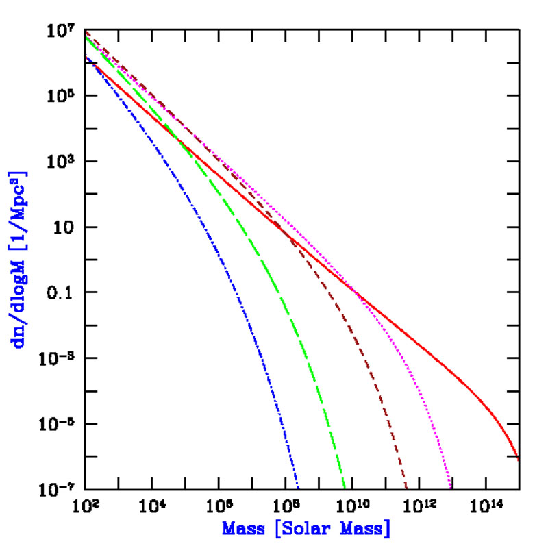 |
Figure 19. Halo mass function at several redshifts: z = 0 (solid curve), z = 5 (dotted curve), z = 10 (short-dashed curve), z = 20 (long-dashed curve), and z = 30 (dot-dashed curve). |
4.2. The Excursion-Set (Extended Press-Schechter) Formalism
The usual Press-Schechter formalism makes no attempt to deal with the correlations between halos or between different mass scales. In particular, this means that while it can generate a distribution of halos at two different epochs, it says nothing about how particular halos in one epoch are related to those in the second. We therefore would like some method to predict, at least statistically, the growth of individual halos via accretion and mergers. Even restricting ourselves to spherical collapse, such a model must utilize the full spherically-averaged density profile around a particular point. The potential correlations between the mean overdensities at different radii make the statistical description substantially more difficult.
The excursion set formalism (Bond et al. 1991
[52])
seeks to
describe the statistics of halos by considering the statistical properties
of  (R),
the average overdensity within some spherical window of characteristic
radius R, as a function of R. While the
Press-Schechter model depends only on the Gaussian distribution of
for one
particular R, the excursion set considers all
R. Again the connection between a value of the linear regime
and the final state is made via the spherical collapse solution, so that
there is a critical value
c (z)
of which is
required for collapse at a redshift z.
(R),
the average overdensity within some spherical window of characteristic
radius R, as a function of R. While the
Press-Schechter model depends only on the Gaussian distribution of
for one
particular R, the excursion set considers all
R. Again the connection between a value of the linear regime
and the final state is made via the spherical collapse solution, so that
there is a critical value
c (z)
of which is
required for collapse at a redshift z.
For most choices of window function, the functions
(R)
are correlated from one R to another such that it is prohibitively
difficult to calculate the desired statistics directly [although Monte
Carlo realizations are possible
[52]].
However, for one particular choice of a window function, the correlations
between different R greatly simplify and many interesting
quantities may be calculated
[52,
212].
The key is to use a k-space top-hat
window function, namely Wk = 1 for all k less
than some critical kc
and Wk = 0 for k >
kc. This filter has a spatial form of
W(r)  j1 (kc r) /
kc r, which implies a volume
6
j1 (kc r) /
kc r, which implies a volume
6 2 /
kc3 or mass
62
2 /
kc3 or mass
62
 b /
kc3. The characteristic radius
of the filter is ~ kc-1, as expected. Note
that in real space,
this window function converges very slowly, due only to a sinusoidal
oscillation, so the region under study is rather poorly localized.
b /
kc3. The characteristic radius
of the filter is ~ kc-1, as expected. Note
that in real space,
this window function converges very slowly, due only to a sinusoidal
oscillation, so the region under study is rather poorly localized.
The great advantage of the sharp k-space filter is that the
difference at a given point between
on one mass
scale and that on
another mass scale is statistically independent from the value on the
larger mass scale. With a Gaussian random field, each
k is Gaussian
distributed independently from the others. For this filter,
 |
(93) |
meaning that the overdensity on a particular scale is simply the sum of the
random variables
k interior to
the chosen kc. Consequently,
the difference between the
(M) on
two mass scales is just the sum of the
k in the
spherical shell between the two
kc, which is independent from the sum of the
k interior to the
smaller kc. Meanwhile, the distribution of
(M) given
no prior information is still a Gaussian of mean zero and variance
 |
(94) |
If we now consider
as a function
of scale kc, we see that we begin from
= 0 at
kc = 0 (M =
)
and then add independently random pieces as kc
increases. This generates a random walk, albeit one whose stepsize
varies with kc. We
then assume that, at redshift z, a given function
(kc
) represents a collapsed mass M corresponding to the
kc where the
function first crosses the critical value
c
(z). With this assumption, we may use the properties of random
walks to calculate the evolution of the mass as a function of redshift.
It is now easy to rederive the Press-Schechter mass function, including the
previously unexplained factor of 2
[52,
212,
382].
The fraction of mass elements included in halos of mass less than
M is just the probability that a random walk remains below
c (z)
for all kc
less than Kc, the filter cutoff appropriate to
M. This probability
must be the complement of the sum of the probabilities that: (a)
(Kc) >
c(z);
or that (b)
(Kc) <
c(z)
but (k'c) >
c(z)
for some k'c < Kc. But these two
cases in fact have equal probability; any random walk belonging to class
(a) may be reflected around its first upcrossing of
c(z)
to produce a walk of class
(b), and vice versa. Since the distribution of
(Kc) is simply Gaussian with variance
2(M),
the fraction of random walks falling into class (a) is simply (1 /
(2
2)1/2)
 c (z)
d exp{-
2 /
22 (M)}.
Hence, the fraction of mass elements
included in halos of mass less than M at redshift z is simply
c (z)
d exp{-
2 /
22 (M)}.
Hence, the fraction of mass elements
included in halos of mass less than M at redshift z is simply
 |
(95) |
which may be differentiated to yield the Press-Schechter mass function. We
may now go further and consider how halos at one redshift are related to
those at another redshift. If we are given that a halo of mass
M2 exists at redshift z2, then we
know that the random function
(kc) for each mass element within the
halo first crosses
(z2)
at kc2 corresponding to M2. Given this
constraint, we may study the distribution of kc where
the function
(kc) crosses other thresholds. It is
particularly easy
to construct the probability distribution for when trajectories first cross
some c
(z1) >
c
(z2) (implying z1 >
z2); clearly this occurs at some kc1
> kc2. This problem reduces to
the previous one if we translate the origin of the random walks from
(kc,
) = (0,0) to
(kc2,
c(z2)).
We therefore find the distribution of halo masses M1
that a mass element
finds itself in at redshift z1 given that it is part
of a larger halo of
mass M2 at a later redshift z2 is
[52,
55])
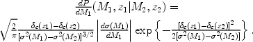 |
(96) |
This may be rewritten as saying that the quantity
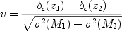 |
(97) |
is distributed as the positive half of a Gaussian with unit variance;
equation (97) may be inverted to find
M1( ).
).
We seek to interpret the statistics of these random walks as those of merging and accreting halos. For a single halo, we may imagine that as we look back in time, the object breaks into ever smaller pieces, similar to the branching of a tree. Equation (96) is the distribution of the sizes of these branches at some given earlier time. However, using this description of the ensemble distribution to generate Monte Carlo realizations of single merger trees has proven to be difficult. In all cases, one recursively steps back in time, at each step breaking the final object into two or more pieces. An elaborate scheme (Kauffmann & White 1993 [195]) picks a large number of progenitors from the ensemble distribution and then randomly groups them into sets with the correct total mass. This generates many (hundreds) possible branching schemes of equal likelihood. A simpler scheme (Lacey & Cole 1993 [212]) assumes that at each time step, the object breaks into two pieces. One value from the distribution (96) then determines the mass ratio of the two branchs.
One may also use the distribution of the ensemble to derive some additional analytic results. A useful example is the distribution of the epoch at which an object that has mass M2 at redshift z2 has accumulated half of its mass [212]. The probability that the formation time is earlier than z1 is equal to the probability that at redshift z1 a progenitor whose mass exceeds M2/2 exists:
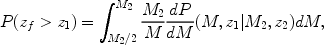 |
(98) |
where dP / dM is given in equation (96). The factor of M2 / M corrects the counting from mass weighted to number weighted; each halo of mass M2 can have only one progenitor of mass greater than M2 / 2. Differentiating equation (98) with respect to time gives the distribution of formation times. This analytic form is an excellent match to scale-free N-body simulations [213]. On the other hand, simple Monte Carlo implementations of equation (96) produce formation redshifts about 40% higher [212]. As there may be correlations between the various branches, there is no unique Monte Carlo scheme.
Numerical tests of the excursion set formalism are quite encouraging. Its
predictions for merger rates are in very good agreement with those measured
in scale-free N-body simulations for mass scales down to around 10% of the
nonlinear mass scale (that scale at which
m = 1), and
distributions of formation times closely match the analytic predictions
[213].
The model appears to be a promising method for tracking the
merging of halos, with many applications to cluster and galaxy formation
modeling. In particular, one may use the formalism as the foundation of
semi-analytic galaxy formation models
[196].
The excursion set formalism may also be used to derive the correlations
of halos in the nonlinear regime
[258].
4.3. Response of Baryons to Nonlinear Dark Matter Potentials
The dark matter is assumed to be cold and to dominate gravity, and so its collapse and virialization proceeds unimpeded by pressure effects. In order to estimate the minimum mass of baryonic objects, we must go beyond linear perturbation theory and examine the baryonic mass that can accrete into the final gravitational potential well of the dark matter.
For this purpose, we assume that the dark matter had already
virialized and produced a gravitational potential
 (r) at a
redshift zvir (with
0 at large distances,
and < 0 inside the
object) and calculate the resulting
overdensity in the gas distribution, ignoring cooling (an assumption
justified by spherical collapse simulations which indicate that
cooling becomes important only after virialization; see Haiman et al. 1996
[168]).
(r) at a
redshift zvir (with
0 at large distances,
and < 0 inside the
object) and calculate the resulting
overdensity in the gas distribution, ignoring cooling (an assumption
justified by spherical collapse simulations which indicate that
cooling becomes important only after virialization; see Haiman et al. 1996
[168]).
After the gas settles into the dark matter potential well, it satisfies the hydrostatic equilibrium equation,
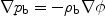 |
(99) |
where pb and
b
are the pressure and mass density
of the gas. At z < 100 the gas temperature is decoupled from the
CMB, and its pressure evolves adiabatically (ignoring atomic or
molecular cooling),
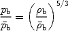 |
(100) |
where a bar denotes the background conditions. We substitute equation (100) into (99) and get the solution,
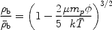 |
(101) |
where  =
=
 b µ
mp / (k
b µ
mp / (k
 b)
is the background gas temperature. If we define Tvir=
-1/3mp
/ k as the virial temperature for a potential
depth -, then the
overdensity of the baryons at the virialization redshift is
b)
is the background gas temperature. If we define Tvir=
-1/3mp
/ k as the virial temperature for a potential
depth -, then the
overdensity of the baryons at the virialization redshift is
 |
(102) |
This solution is approximate for two reasons: (i) we assumed that the gas is stationary throughout the entire region and ignored the transitions to infall and the Hubble expansion at the interface between the collapsed object and the background intergalactic medium (henceforth IGM), and (ii) we ignored entropy production at the virialization shock surrounding the object. Nevertheless, the result should provide a better estimate for the minimum mass of collapsed baryonic objects than the Jeans mass does, since it incorporates the nonlinear potential of the dark matter.
We may define the threshold for the collapse of baryons by the
criterion that their mean overdensity,
b, exceeds a
value of 100, amounting to > 50% of the baryons that would
assemble in the absence of gas pressure, according to the spherical
top-hat collapse model. Equation (102) then
implies that Tvir > 17.2
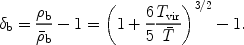
.
As mentioned before, the gas temperature evolves at z < 160
according to the relation
 170 [(1 + z)
/ 100]2 K. This implies
that baryons are overdense by
b > 100
only inside halos with
a virial temperature Tvir > 2.9 ×
103 [(1 + z) / 100]2 K. Based on the top-hat
model, this implies a minimum halo mass for baryonic objects of
170 [(1 + z)
/ 100]2 K. This implies
that baryons are overdense by
b > 100
only inside halos with
a virial temperature Tvir > 2.9 ×
103 [(1 + z) / 100]2 K. Based on the top-hat
model, this implies a minimum halo mass for baryonic objects of
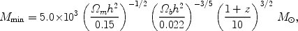 |
(103) |
where we consider sufficiently high redshifts so that
mz
1. This minimum mass is coincidentally almost identical to the naive
Jeans mass calculation of linear theory in equation (62)
despite the fact that it incorporates shell crossing by the dark
matter, which is not accounted for by linear theory. Unlike the Jeans
mass, the minimum mass depends on the choice for an overdensity
threshold [taken arbitrarily as
b > 100 in
equation (103)]. To estimate the minimum halo mass which
produces any significant accretion we set, e.g.,
b = 5,
and get a mass which is lower than Mmin by a factor of 27.
Of course, once the first stars and quasars form they heat the surrounding IGM by either outflows or radiation. As a result, the Jeans mass which is relevant for the formation of new objects changes [148, 152]). The most dramatic change occurs when the IGM is photo-ionized and is consequently heated to a temperature of ~ (1 - 2) × 104 K.