


We will begin with a discussion of the important observational techniques that we use to obtain information about the star-forming ISM. This will naturally lead us to review some of the important radiative transfer physics that we need to keep in mind to understand the observations. Because the interstellar clouds that form stars are generally cold, most (but not all) of these techniques require on infrared, sub-millimeter, and radio observations.
Hydrogen is the most abundant element, and when it is in the form of free atomic hydrogen, it is relatively easy to observe. Hydrogen atoms have a hyperfine transition at 21 cm (1.4 GHz), associated with a transition from a state in which the spin of the electron is parallel to that of the proton to a state where it is anti-parallel. The energy associated with this transition is << 1 K, so even in cold regions it can be excited. This line is seen in the Milky Way and in many nearby galaxies.
However, at the high densities where stars form, hydrogen tends to be molecular rather than atomic, and H2 is extremely hard to observe directly. To understand why, we must review the quantum structure of H2. A diatomic molecule like H2 has three types of excitation: electronic (corresponding to excitations of one or more of the electrons), vibrational (corresponding to vibrational motion of the two nuclei), and rotational (corresponding to rotation of the two nuclei about the center of mass). Generally electronic excitations are highest in energy scale, vibrational are next, and rotational are the lowest in energy.
For H2, the first excited state, the J = 1 rotational
state, is 100-200 K above the ground state.
This energy gap between the ground state and the first excited state is
far larger than for any other simple molecule, and the underlying reason
for this large energy is the low mass of hydrogen. For a quantum
oscillator or rotor the level spacing varies with reduced mass as
m-1/2. Since the dense ISM
where molecules form is often also cold, T ~ 10 K (as we discuss
later), almost no molecules will be in this
excited state. However, it gets even worse: H2 is a
homonuclear molecule, which means that it has zero electric dipole
moment. As a result, electric dipole transitions do not occur, and
radiative transitions that change J by 1 are electric
dipoles. This means that there is no J = 1
 0 emission.
Instead, the lowest-lying transition
is the J = 2
0 quadrupole. This is very
weak, because it's a quadrupole. More importantly, however, the
J = 2 state is 511 K above the ground state. This means that, for a
population in equilibrium at a temperature of 10 K, the fraction of
molecules in the J = 2 state is ~ e-10/500
0 emission.
Instead, the lowest-lying transition
is the J = 2
0 quadrupole. This is very
weak, because it's a quadrupole. More importantly, however, the
J = 2 state is 511 K above the ground state. This means that, for a
population in equilibrium at a temperature of 10 K, the fraction of
molecules in the J = 2 state is ~ e-10/500
 10-22! In
effect, in a molecular cloud there are simply no H2 molecules
in states capable of emitting.
10-22! In
effect, in a molecular cloud there are simply no H2 molecules
in states capable of emitting.
The conclusion of this analysis is that, for typical conditions in star-forming clouds, we cannot observe the most abundant species, H2, in emission. Instead, we are forced to observe proxies instead. (One can observe H2 in absorption against background sources, but this is possible only in special circumstances.)
One proxy we can use, which is perhaps the most straightforward
conceptually, is dust. Interstellar gas clouds are always mixed with
dust, and the dust grains emit thermal radiation which we can
observe. They also absorb background starlight, and we observe that
absorption too. The advantage of dust grains is that, since they are
solid particles, the can absorb or emit continuum radiation, which the
gas cannot. Consider a cloud of gas of mass density
 mixed with dust
grains at a temperature T. The gas-dust mixture has a specific
opacity
mixed with dust
grains at a temperature T. The gas-dust mixture has a specific
opacity 
 to radiation at
frequency
. Although the vast majority
of the mass is in gas rather than dust, the opacity will be almost
entirely due to the dust grains except for frequencies that happen to
match the resonant absorption frequencies of atoms and molecules in the
gas.
to radiation at
frequency
. Although the vast majority
of the mass is in gas rather than dust, the opacity will be almost
entirely due to the dust grains except for frequencies that happen to
match the resonant absorption frequencies of atoms and molecules in the
gas.
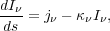
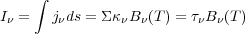
Radiation passing through the cloud is governed by the equation of radiative transfer:
 |
(1) |
where
I
is the radiation intensity, and we integrate along a path through the
cloud. The emissivity for gas of opacity
that is in
local thermodynamic equilibrium (LTE) is
j
=
B(T), where
j
has units of erg s-1 cm-3 sr-1
Hz-1, i.e. it describes the number of ergs emitted in 1
second by 1 cm3 of gas into a solid angle of 1 sr in a
frequency range of 1 Hz, and
 |
(2) |
is the Planck function.
Generally we look for emission at submillimeter wavelengths, and for
absorption at near infrared wavelengths. In the sub-mm typical opacities
are
~ 0.01
cm2 g-1. Since essentially no interstellar cloud
has a surface density > 100 g cm-2, absorption of
radiation from the back of the cloud by gas in front of it is completely
negligible. Thus, we can set
I
to zero in the transfer equation, and integrate trivially:
 |
(3) |
where  =
=
 ds is
the surface density of the cloud and
ds is
the surface density of the cloud and
 =
is the optical
depth of the cloud at frequency .
Thus if we observe the intensity of emission from dust grains in a
cloud, we determine the product of the optical depth and the Planck
function, which is determined solely by the observing frequency and the
gas temperature. If we know the temperature and the properties of the
dust grains, we can therefore determine the column density of the gas in
the cloud in each telescope beam.
=
is the optical
depth of the cloud at frequency .
Thus if we observe the intensity of emission from dust grains in a
cloud, we determine the product of the optical depth and the Planck
function, which is determined solely by the observing frequency and the
gas temperature. If we know the temperature and the properties of the
dust grains, we can therefore determine the column density of the gas in
the cloud in each telescope beam.
Conversely, if we are looking for absorption in the near-IR, we have a
background star that emits light that enters the cloud with intensity
I,0. The
cloud itself emits negligibly in the near-IR, because
h >> kT,
so the exponential factor in the denominator of the Planck function is
huge. Thus we can drop the
j
term in the transfer equation, and the solution is again trivial:
 |
(4) |
By measuring the optical depth at several frequencies, and knowing the
intrinsic frequency-dependence of
I,0 for
stars, we can figure out the optical depth and thus the column density.
These mapping techniques allow us to obtain extremely detailed maps of nearby molecular clouds. Figure 1 shows a spectacular example. Unfortunately, these techniques are generally not usable for extragalactic observations. The resolution and sensitivity of sub-mm telescopes is not sufficient to allow us to see individual clouds in emission, and the problem of knowing which stars are behind or in front of a given gas cloud at extragalactic distances prevents us from making good measurements in absorption. Both of these limitations may be eased by future telescopes, but for now dust observations of individual clouds are generally limited to the Milky Way.
 |
Figure 1. A map of the Pipe Nebula obtained with near-infrared absorption measurements. Color indicates visual extinction, which is proportional to column density. Reprinted with permission from [3]. |
Much of what we know about star forming gas comes from observations of molecular line emission. These are usually the most complex measurements in terms of the modeling and required to understand them. However, they are also by far the richest in terms of the information they provide. They are also among the most sensitive, since the lines can be very bright compared to continuum emission. Indeed, almost everything we know about giant molecular clouds outside of our own galaxy comes from studying emission in the rotational lines of the CO molecule. The CO molecule, since it is much more massive than H2, has its lowest rotational state only 5.5 K above ground, low enough to be excited even at GMC temperatures. Since C and O are two of the most common elements in the ISM beyond H and He, CO molecules are abundant and the lines are bright.
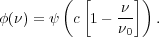
The simplest line-emitting system is an atom or molecule with exactly two energy states, but this example contains most of the concepts we will need. We'll explore how that works first, then consider more complex, realistic molecules. Consider an atom or molecule of species X with two states that are separated by an energy E. Suppose we have a gas of such particles with number density nX at temperature T. The number density of atoms in the ground state is n0 and the number density in the excited state is n1. At first suppose that this system does not radiate. In this case collisions between the atoms will eventually bring the two energy levels into thermal equilibrium. In that case, what are n0 and n1?
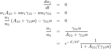
They just follow a Boltzmann distribution, so n1 / n0 = e-E / kT, and thus we have n0 = nX / Z and n1 = nX e-E / kT / Z, where Z = 1 + e-E / kT is the partition function. Gas with such a distribution of level populations is said to be in LTE. Now let's consider radiative transitions between these states. There are three processes: spontaneous emission, stimulated emission, and absorption, which are described by the three Einstein coefficients. For simplicity we'll start by neglecting all but spontaneous emission. This is sometimes a good approximation in the interstellar medium, since in many cases the ambient radiation field is too weak for stimulated emission or absorption to be important.
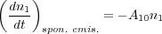
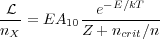
A particle in the excited state can spontaneously emit a photon and decay to the ground state. The rate at which this happens is described by the Einstein coefficient A10, which has units of s-1. Its meaning is simply that a population of n1 atoms in the excited state will decay to the ground state by spontaneous emission at a rate
 |
(5) |
atoms per cm3 per s, or equivalently that the e-folding time for decay is 1 / A10 seconds.
For the molecules we'll be spending most of our time talking about, decay times are typically at most a few centuries, which is short compared to pretty much any time scale associated with star formation. Thus if spontaneous emission were the only process at work, all molecules would quickly decay to the ground state and we wouldn't see any emission. However, in the dense interstellar environments where stars form, collisions occur frequently enough to create a population of excited molecules. Of course collisions involving excited molecules can also cause de-excitation, with the excess energy going into recoil rather than into a photon.
Since hydrogen molecules are almost always the most abundant species in the dense regions we're going to think about, with helium second, we can generally only consider collisions between our two-level atom and those partners. For the purposes of this exercise, we'll ignore everything but H2. The rate at which collisions cause transitions between states is a horrible quantum mechanical problem. We cannot even confidently calculate the energy levels of single isolated molecules except in the simplest cases, let alone the interactions between two colliding ones at arbitrary velocities and relative orientations. Exact calculations of collision rates are generally impossible. Instead, we either make due with approximations (at worst), or we try to make laboratory measurements. Things are bad enough that, for example, we often assume that the rates for collisions with H2 molecules and He atoms are related by a constant factor.
Fortunately, as astronomers we generally leave these problems to chemists, and instead do what we always do: hide our ignorance behind a parameter. We let the rate at which collisions between species X and H2 molecules induce transitions from the ground state to the excited state be
 |
(6) |
where n is the number density of H2 molecules
(not the number density of species X) and
 01
has units of cm3 s-1. In general
01
will be a function of the gas kinetic temperature T, but not of
n (unless n is so high that three-body processes start to
become important, which is almost never the case in the ISM). The
corresponding rate coefficient for collisional de-excitation is
10,
and the collisional de-excitation rate is
01
has units of cm3 s-1. In general
01
will be a function of the gas kinetic temperature T, but not of
n (unless n is so high that three-body processes start to
become important, which is almost never the case in the ISM). The
corresponding rate coefficient for collisional de-excitation is
10,
and the collisional de-excitation rate is
 |
(7) |
Collections of collision rate coefficients for common molecules can be found in the extremely useful Leiden Atomic and Molecular Database 1 [4].
A little thought will convince you that
01
and
10
must have a specific relationship. Consider an extremely optically thick
region where so few photons escape that radiative processes are not
significant. If the gas is in equilibrium then we have
 |
(8) (9) |
However, we also know that the equilibrium distribution is a Boltzmann distribution, so n1 / n0 = e-E / kT. Thus we have
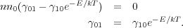 |
(10) (11) |
This argument applies equally well between a pair of levels even for a complicated molecule with many levels instead of just 2. Thus, we only need to know the rate of collisional excitation or de-excitation between any two levels to know the reverse rate.
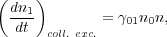
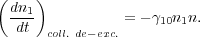
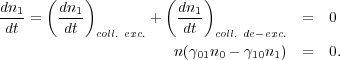
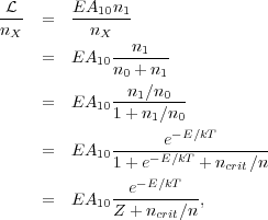
We are now in a position to write down the full equations of statistical equilibrium for the two-level system. In so doing, we will see that we can immediately use line emission to learn a great deal about the density of gas. In equilibrium we have
 |
(12) (13) (14) (15) (16) |
This physical meaning of this expression is clear. If radiation is
negligible compared to collisions, i.e. A10 <<
10 n, then the ratio of level
populations approaches the Boltzmann ratio e-E /
kT. As radiation becomes more important, i.e.
A10/(10 n) get larger, the fraction in the
upper level drops - the level population is sub-thermal. This is because
radiative decays remove molecules from the upper state much faster than
collisions re-populate it.
Since the collision rate depends on density and the radiative decay rate
does not, the balance between these two processes depends on
density. This make it convenient to introduce a critical density
ncrit, defined by ncrit =
A10 /
10, so that
 |
(17) |
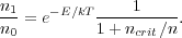
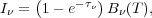
At densities much larger than ncrit, we expect the level population to be close to the Boltzmann value, and at densities much smaller than ncrit we expect the upper state to be under-populated relative to Boltzmann. ncrit itself is simply the density at which radiative and collisional de-excitations out of the upper state occur at the same rate.
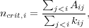
For real molecules or atoms with more than two states, the critical density for state i can be generalized to
 |
(18) |
i.e. the critical density is simply the sum of the Einstein A's for all levels less than i, divided by the sum of the collision rate coefficients for transitions from level i to all levels less than i. The condition for equilibrium is
 |
(19) |
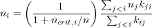
This is a series of linear equations (one for each level i) that can be solved to give the level populations. We could write down an exact solution in terms of a matrix inversion, but it's more illuminating just to notice how the solution will have to behave. For n >> ncrit,i, the leading term in parentheses goes to unity, and the relationships between the different level populations ni are just determined by the collision rate coefficients kij - the Einstein coefficient drops out of the problem. In this case, the level populations go to the Boltzmann distribution. For n << ncrit,i, the leading term in parentheses is smaller than unity, and higher levels are underpopulated relative to the Boltzmann distribution. Thus the behavior is qualitatively similar to the two-level atom.
2.2. Molecular Cloud Properties from Molecular Lines
Molecular lines, as we have seen, are a rather complicated way to observe things, since the emission we get out depends on many factors. However, we can turn this to our advantage. The complexity of the molecular line emission process can be exploited to tell us all sorts of things about molecular clouds. Indeed, they form the basis of most of our knowledge of cloud properties. For the rest of this section we'll mostly go back to our two-level particle for simplicity, since the procedures for multi-level particles are analogous but more mathematically cumbersome.
First of all, let's consider the rate of energy emission per molecule from a molecular line. This is easy once we know the level population:
 |
(20) (21) (22) (23) (24) |
where again Z is the partition function. It is instructive to think about how this behaves in the limiting cases n << ncrit and n >> ncrit. In the limit n >> ncrit, the partition function Z dominates the denominator, and we get L / nX = E A10 e-E / kTZ. This is just the energy per spontaneous emission times the spontaneous emission rate times the fraction of the population in the upper state when the gas is in statistical equilibrium. This is density-independent, so this means that at high density you just get a fixed amount of emission per molecule of the emitting species. The total luminosity is just proportional to the number of emitting molecules.
For n << ncrit, the second term dominates the denominator, and we get
 |
(25) |
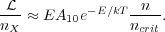
Thus at low density each molecule contributes an amount of light that is proportional to the ratio of density to critical density. Note that this is the ratio of collision partners, i.e. of H2, rather than the density of emitting molecules. The total luminosity varies as this ratio times the number of emitting molecules. Figure 2 shows an example of this behavior for the first three rotational transitions of CO.
 |
|
Figure 2. Emitted luminosity per CO
molecule as a function of H2 density n, for the
J = 1 |
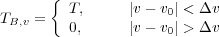
The practical effect of this is that, at densities below the critical density, emission from a molecular line is often unobservably small. Even if it can be observed, emission from gas below the critical density is likely to be dwarfed by emission from gas at or above the critical density. This means that observing molecular lines often immediately tells us about the volume density of the gas! In effect, a measurement of the luminosity of a particular line tells us something like the total mass of gas that is dense enough to excite that line. If we observe a cloud in many different molecular lines with different critical densities, we can deduce the density distribution within that cloud. Analysis of this sort indicates that the bulk of the material in molecular clouds is at densities n ~ 100 cm-3, while small amounts of mass reach much higher densities.
As a caution I should mention that this is computed for optically thin emission. If the line is optically thick, you can no longer ignore stimulated emission and absorption processes, and not all emitted photons will escape from the cloud. CO is usually optically thick. The effect of optical thickness is to reduce the effective critical density. This is because trapping of photons within the cloud means that not every spontaneously-emitted photon escapes the cloud, which has an effect like like lowering the Einstein A.
2.2.2. Velocity and temperature inference
We can also use molecular lines to infer the velocity and temperature
structure of gas if the line in question is optically thin, meaning that
we can neglect absorption. For an optically thin line, the width of the
line is determined primarily by the velocity distribution of the
emitting molecules. The physics here is extremely simple. Suppose we
have gas along our line of sight with a velocity distribution
 (v), i.e. the
fraction of gas with velocities between v and v +
dv is (v)
dv, and
-
(v), i.e. the
fraction of gas with velocities between v and v +
dv is (v)
dv, and
- (v) dv =
0. For an optically thin line, in the limit where natural and
pressure-broadening of lines is negligible, we can think of emission
producing a delta function in frequency in the rest frame of the
gas. There is a one-to-one mapping between velocity and frequency. Thus
emission from gas moving at a frequency v relative to us along
our line of sight produces emission at a frequency
(v) dv =
0. For an optically thin line, in the limit where natural and
pressure-broadening of lines is negligible, we can think of emission
producing a delta function in frequency in the rest frame of the
gas. There is a one-to-one mapping between velocity and frequency. Thus
emission from gas moving at a frequency v relative to us along
our line of sight produces emission at a frequency
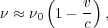 |
(26) |
where 0 is the
central frequency of the line in the molecule's rest frame, and we
assume v/c << 1.
In this case the line profile is described trivially by
 |
(27) |
We can measure  () directly, and
this immediately tells us the velocity distribution
(v). In general the
velocity distribution of the gas
(v) is produced by a
combination of thermal and non-thermal motions. Thermal motions arise
from the Maxwellian velocity distribution of the gas, and produce a
Maxwellian profile
()
() directly, and
this immediately tells us the velocity distribution
(v). In general the
velocity distribution of the gas
(v) is produced by a
combination of thermal and non-thermal motions. Thermal motions arise
from the Maxwellian velocity distribution of the gas, and produce a
Maxwellian profile
()
 e-(-cen)2 /
 2. Here
cen is the central
frequency of the line, which is
cen =
0 (1 -
2. Here
cen is the central
frequency of the line, which is
cen =
0 (1 -
 / c), where
is the mean velocity of
the gas along our line of sight. The width is
=
(kT / µ)1/2 / c, where T is
the gas temperature and µ is the mean mass of the emitting
molecule. This is just the 1D Maxwellian distribution.
/ c), where
is the mean velocity of
the gas along our line of sight. The width is
=
(kT / µ)1/2 / c, where T is
the gas temperature and µ is the mean mass of the emitting
molecule. This is just the 1D Maxwellian distribution.
Non-thermal motions involve bulk flows of the gas, and can produce a variety of velocity distributions depending how the cloud is moving. Unfortunately even complicated motions often produce distributions that look something like Maxwellian distributions, just because of the central limit theorem: if you throw together a lot of random junk, the result is usually a Gaussian distribution.
Determining whether a given line profile reflects predominantly thermal or non-thermal motion requires that we have a way of estimating the temperature independently. This can often be done by observing multiple lines of the same species. Our expression
 |
(28) |
shows that the luminosity of a particular optically thin line is a function of the temperature T, the density n, and the number density of emitting molecules nX. If we observe three transitions of the same molecule, then we have three equations in three unknowns and we can solve for n, nX, and T independently. Certain molecules, because of their level structures, make this technique particularly clean. The most famous example of this is ammonia, NH3.
Measurements of this sort show that typical molecular clouds have
velocity dispersions of several km s-1, but very low
temperatures of only ~ 10 K. This is significant because the sound
speed for H2 molecules at 10 K is cs =
(k T / mH2)1/2
0.2 km
s-1. Thus the observed linewidths indicate that the typical
velocities of material inside a GMC are supersonic by factors of ~
10. This has important implications that we will explore below.
The last thing we routinely infer from line observations is total masses
of clouds. In this case we usually want to pick a line that is quite
optically thick, such as CO J = 1
0.
Other commonly-used lines include CO J = 2
1,
13CO J = 1
0 and
J = 2 1,
and HCN J = 1 0.
The main motivation for using an optically thick line is that these tend
to be nice and bright, so they're observable in external galaxies, or at
long distances within our galaxy.
The challenge for an optically thick line is how to infer a mass, given
that we're really only seeing the surface of a cloud. At first blush
this shouldn't be possible - after all, I cannot infer how thick a wall
is by seeing its surface. The reason it is possible is that molecular
clouds are not like walls. Even at their surfaces they carry information
about their full mass. To see why this is, consider optically thick line
emission from a cloud of mass M and radius R at
temperature T. The mean column density is N = M /
(µ  R2), where µ = 3.9 × 10⁻²⁴
g is the mass per H2 molecule.
R2), where µ = 3.9 × 10⁻²⁴
g is the mass per H2 molecule.
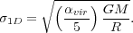
Suppose this cloud is in virial balance between kinetic energy and
gravity, so that its kinetic energy is half its potential energy (we'll
discuss this more in the context of the virial theorem in the next
section). The gravitational-self energy is
 = -a
GM2 / R, where a is a constant of order
unity that depends on the cloud's geometry and internal mass
distribution. For a uniform sphere a = 3/5. The kinetic energy is
= -a
GM2 / R, where a is a constant of order
unity that depends on the cloud's geometry and internal mass
distribution. For a uniform sphere a = 3/5. The kinetic energy is
 = (3/2)
M1D2, where
1D is the one
dimensional velocity dispersion, including both thermal and non-thermal
components. We define the virial ratio as
= (3/2)
M1D2, where
1D is the one
dimensional velocity dispersion, including both thermal and non-thermal
components. We define the virial ratio as
 |
(29) |
For a uniform sphere, which has a = 3/5, this definition implies
 vir =
2 /
||. Thus
vir = 1
corresponds to the ratio of kinetic to gravitational energy in a uniform
sphere of gas in virial equilibrium between internal motions and
gravity. In general we expect that
vir
1 in any object
supported primarily by internal turbulent motion, even if its mass
distribution is not uniform. Re-arranging this definition, we have
vir =
2 /
||. Thus
vir = 1
corresponds to the ratio of kinetic to gravitational energy in a uniform
sphere of gas in virial equilibrium between internal motions and
gravity. In general we expect that
vir
1 in any object
supported primarily by internal turbulent motion, even if its mass
distribution is not uniform. Re-arranging this definition, we have
 |
(30) |
To see why this is relevant for the line emission, consider the total frequency-integrated intensity that the line will emit. The emission will be dominated by gas with a density above the critical density, for the reason we just discussed. This gas is close to LTE, so its emissivity is given by the Planck function times its opacity. In this case the solution to the transfer equation is
 |
(31) |
so integrating over frequency we get
 |
(32) |
By assumption the optical depth at line center is
0 >> 1, and
for a Gaussian line profile the optical depth at frequency
is
 |
(33) |
Since the integrated intensity depends on the integral of
over frequency,
and the frequency-dependence of
is determined
by
1D, we
therefore expect that the integrated intensity will depend on
1D.
To get a sense of how this dependence will work, let us adopt a very
simplified yet schematically correct form for
. We will take
the opacity to be a step function, which is infinite near line center
and drops sharply to 0 far from line center. The frequency at which this
transition happens will be set by the condition
=1, which gives
 |
(34) |
The corresponding range in Doppler shift is
 |
(35) |
For this step-function form of
, the emitted
brightness temperature is trivial to compute. At velocity v, the
brightness temperature is
 |
(36) |
If we integrate this over all velocities of emitting molecules, we get
 |
(37) |
Thus, the velocity-integrated brightness temperature is simply
proportional to
1D. The
dependence on the line-center optical depth is generally negligible,
since that quantity enters only as the square root of the log.
Now let us consider the amount of emission we get per unit column density within our telescope beam. We define this quantity as X, and we have
 |
where n = 3M /
(4 R3) is
the number density of the cloud, and the factor of 105 comes
from the fact that we're measuring ICO in km
s-1 rather than cm s-1. To the extent that all
molecular clouds have comparable volume densities on large scales and
are virialized, this suggests that there should be a roughly constant CO
X factor. If we plug in T = 10 K, n = 100 cm-3,
vir = 1, and
0 = 100, this
gives XCO = 5 × 1019 cm-2
(K km s-1)-1.
This is quite a result: it means that we have inferred the mass of a molecular cloud simply by measuring the luminosity it emits in a particular optically thick line. Of course this calculation has a few problems - we have to assume a volume density, and there are various fudge factors like a floating around. Moreover, we had to assume virial balance between gravity and internal motions. This implicitly assumes that both surface pressure and magnetic fields are negligible, which they may not be. Making this assumption would necessarily make it impossible to independently check whether molecular clouds are in fact in virial balance between gravity and turbulent motions.
In practice, the way we get around these problems is by determining X
factors by empirical calibration. We generally do this by attempting to
measure the total gas column density by some tracer that measures all
the gas along the line of sight, and then subtracting off the observed
atomic gas column - the rest is assumed to be molecular. One way of
doing this is measuring
rays
emitted by cosmic rays interacting with the ISM. The
ray
emissivity is simply proportional to the number density of hydrogen
atoms independent of whether they are in atoms or molecules (since the
cosmic ray energy is very large compared to any molecular energy
scales). Once produced the
rays
travel to Earth without significant attenuation, so the
ray
intensity along a line of sight is simply proportional to the total
hydrogen column. Another way is to measure the infrared emission from
dust grains along the line of sight, which gives the total dust
column. This is then converted to a mass column using a dust to gas
ratio. Yet a third method is to observe a cloud in multiple molecular
lines, some of which are optically thin and some of which are thick, and
use the multiple lines in an attempt to determine the absolute mass.
Using any of these techniques in the Milky Way gives X
2 ×
1020 cm-2 (K km s-1)-1 for
the Milky Way, with roughly a factor of 2 scatter on either side
depending on the technique used and the assumptions made
[5,
6,
7,
8].
These numbers are roughly consistent with our simple model, and the fact
that several independent techniques give results that match to a factor
of 2 gives us some confidence that the method works.
From this sort of analysis we learn that most of the molecular mass in
our galaxy and in similar nearby galaxies is organized into giant clouds
with masses of ~ 104 - 106
M [9].
[9].
1 http://www.strw.leidenuniv.nl/~moldata/ Back.