3. PHYSICAL PROCESSES IN MOLECULAR CLOUDS

3.1. Heating and cooling proceses

The temperature in molecular clouds is set mostly by radiative processes - adiabatic heating and cooling associated with hydrodynamic motions is generally negligible, as we will show in a moment. Thus we have to consider how clouds can gain and loose heat by radiation. A full treatment of this problem necessarily involves numerical calculations, but we can derive some basic results quite simply.

3.1.1. Heating by cosmic rays

In the bulk of the interstellar medium the main source of heating is starlight. However, typical molecular clouds have visual extinctions A_V ~ 5, which means that starlight in the interior is reduced to a few percent of the mean interstellar value at visible wavelengths, and to much less than a percent of the interstellar value at the ultraviolet wavelengths that produce most heating. Thus, we can generally neglect starlight as a source of heat (except very near young stars forming within the cloud).

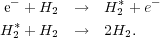
Instead, over the bulk of a molecular cloud's volume, the main source of heating is cosmic rays: relativistic particles accelerated in shocks that are able to penetrate into GMC interiors. How much heat do cosmic rays produce? To answer this question, we must first determine the mechanism by which the gas is heated. The first step in such a heating chain is the interaction of a cosmic ray with an electron, which knocks the electron off a molecule:

(38)

The free electron's energy depends only weakly on the CR's energy, and is typically ~ 30 eV.

The electron cannot easily transfer its energy to other particles in the gas directly, because its tiny mass guarantees that most collisions are elastic and transfer no energy to the impacted particle. However, the electron also has enough energy to ionize or dissociate other hydrogen molecules, which provides an inelastic reaction that can convert some of its 30 eV to heat. Secondary ionizations do indeed occur, but in this case almost all the energy goes into ionizing the molecule (15.4 eV), and the resulting electron has the same problem as the first one: it cannot effectively transfer energy to the much more massive protons.

Instead, it is secondary dissociations and excitations that wind up being the dominant energy channels. The former reaction is

(39)

In this reaction any excess energy in the electron beyond what is needed to dissociate the molecule (4.5 eV) goes into kinetic energy of the two recoiling hydrogen atoms, and the atoms, since they are massive, can then efficiently share that energy with the rest of the gas. Alternately, an electron can hit a hydrogen molecule and excite it without dissociating it. The hydrogen molecule then collides with another hydrogen molecule and collisionally de-excites, and the excess energy again goes into recoil, where it is efficiently shared. The reaction is

(40) (41)

Summing over all possible transfer channels, and including heating by secondary ionizations too, the energy yield per primary cosmic ray ionization is in the range 7-20 eV [10, 11], depending on the density. These figures are slightly uncertain.

Combining this with the primary ionization rate for cosmic rays in the Milky Way, which is observationally-estimated to be about 2 × 10^-17 s^-1 per H nucleus [12], this gives a total heating rate per H nucleus

(42)

The heating rate per unit volume is _CR n, where n is the number density of H nuclei (= 2 × the density of H molecules).

3.1.2. CO cooling

In molecular clouds there are two main cooling processes: molecular lines and dust radiation. Dust can cool the gas efficiently because dust grains are solids, so they are thermal emitters. However, dust is only able to cool the gas if collisions between dust grains and hydrogen molecules occur often enough to keep them thermally well-coupled. Otherwise the grains cool off, but the gas stays hot. The density at which grains and gas become well-coupled is around 10⁴ cm^-3 [13], which is higher than the typical density in a GMC, so we won't consider dust cooling further at this point. We'll return to it in the next section when we discuss collapsing objects, where the densities do get high enough for dust cooling to be important.

The remaining cooling process is line emission, and by far the most important molecule for this purpose is CO, due to its abundance and its ability to radiate even at low temperatures and densities. The physics is fairly simple. CO molecules are excited by inelastic collisions with hydrogen molecules, and such collisions convert kinetic energy to potential energy within the molecule. If the molecule de-excites radiatively, and the resulting photon escapes the cloud, the cloud loses energy and cools.

Let us make a rough attempt to compute the cooling rate via this process. As we mentioned in the last section, a diatomic molecule like CO can be excited rotationally, vibrationally, or electronically. At the low temperatures found in molecular clouds, usually only the rotational levels are important. These are characterized by an angular momentum quantum number J, and each level J has a single allowed radiative transition to level J - 1. Larger J transitions are strongly suppressed because they require emission of multiple photons to conserve angular momentum.

Unfortunately the CO cooling rate is quite difficult to calculate, because the lower CO lines are all optically thick. A photon emitted from a CO molecule in the J = 1 state is likely to be absorbed by another one in the J = 0 state before it escapes the cloud, and if this happens that emission just moves energy around within the cloud and provides no net cooling. The cooling rate is therefore a complicated function of position within the cloud - near the surface the photons are much more likely to escape, so the cooling rate is much higher than deep in the interior. The velocity dispersion of the cloud also plays a role, since large velocity dispersions Doppler shift the emission over a wider range of frequencies, reducing the probability that any given photon will be resonantly re-absorbed before escaping.

In practice this means that CO cooling rates usually have to be computed numerically, and will depend on the cloud geometry if we want accuracy to better than a factor of ~ 2. However, we can get a rough idea of the cooling rate from some general considerations. The high J levels of CO are optically thin, since there are few CO molecules in the J - 1 states capable of absorbing them, so photons they emit can escape from anywhere within the cloud. However, the temperatures required to excite these levels are generally high compared to those found in molecular clouds, so there are few molecules in them, and thus the line emission is weak. Moreover, the high J levels also have high critical densities, so they tend to be sub-thermally populated, further weakening the emission.

On other hand, low J levels of CO are the most highly populated, and thus have the highest optical depths. Molecules in these levels produce cooling only if they are within one optical depth the cloud surface. Since this restricts cooling to a small fraction of the cloud volume (typical CO optical depths are many tens for the 1 0 line), this strongly suppresses cooling.

The net effect of combining the suppression of low J transitions by optical depth effects and of high J transitions by excitation effects is that cooling tends to be dominated a the single line produced by the lowest J level for which the line is not optically thick. This line is marginally optically thin, but is kept close to LTE by the interaction of lower levels with the radiation field. Which line this is depends on the column density and velocity dispersion of the cloud, and detailed calculations show that for typical GMC properties it is generally around J = 5.

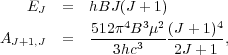
If we assume this dominant cooling level is in LTE, the cooling rate per H nucleus is simply the number of CO molecules per H nucleus times the fraction of molecules in the relevant level, times the emission rate from that level, times the energy per photon:

(43)

where Z is the partition function and x_CO is the ratio of CO molecules to H nuclei. Note that the factor of 2J + 1 is the degeneracy of level J. For a quantum rotator the Einstein A's and energy levels obey

(44) (45)

where B is the rotation constant of the molecule and µ is its electric dipole moment. For CO, B = 57 GHz and µ = 0.112 Debye.

Plugging these values in, for J = 5 4 at T = 10 K we get _CO = 1.3 × 10^-27 erg s^-1 per H nucleus. If we equate the cooling rate to the cosmic ray heating rate of 10^-27 erg s^-1, which is independent of temperature, we find that heating and cooling balance at T 10 K, in good agreement with what we observe. Note that the density does not enter into this, since both and _CO are proportional to density. Thus we expect the equilibrium temperature to be close to density-independent. Due to the exponential dependence, the cooling rate is very temperature-sensitive. If we increase the temperature by a factor of 2, _CO rises by a factor of 30, to about 4 × 10^-26 erg s^-1. Thus it requires a lot of change in heating rate to raise the temperature appreciably.

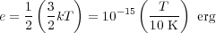
It is also instructive to consider the timescales implied by these cooling rates. The gas thermal energy per H nucleus is

(46)

for a monatomic gas - and H₂ acts like a monatomic gas at low temperature because its rotational degrees of freedom cannot be excited. The factor of 1/2 comes from 2 H nuclei per H₂ molecule. The characteristic cooling time is t_cool = e / _CO. Suppose we have gas that is mildly out of equilibrium, say T = 20 K instead of T = 10 K. The heating and cooling are far out of balance, so we can ignore heating completely compared to cooling. At the cooling rate of _CO = 4 × 10^-26 erg s^-1 for 20 K gas, t_cool = 1.6 kyr. In contrast, the crossing time for a molecular cloud is t_cr = L / ~ 7 Myr for L = 30 pc and = 4 km s^-1. The conclusion of this analysis is that radiative effects happen on time scales much shorter than mechanical ones. Mechanical effects, such as the heating caused by shocks, simply cannot push the gas any significant way out of radiative equilibrium.

3.2. Flows in Molecular Clouds

Now that we have satisfied ourselves that the gas in molecular clouds is, for the most part, kept rigidly fixed at a low temperature, let us consider what that implies about the flows of gas in molecular clouds. In the process we will define four important dimensionless numbers that characterize the flow, two each for the magnetic and non-magnetic cases.

3.2.1. Equations of Motion

We begin by writing down the basic equations of magnetohydrodynamics that govern flows in molecular clouds. There are three such equations in our case:

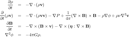(47) (48) (49) (50)

The quantities here are the density , the velocity v, the pressure P, the magnetic field B, the gravitational potential , the kinematic viscosity , and the magnetic resistivity . Note that, in general, can be a tensor, and the colon represents tensor contraction. Since the temperature is fixed by radiative effects, the equation of state is simple. We characterize the temperature by a sound speed c_s, which is related to the pressure by

(51)

Physically, the first equation represents conservation of matter. It states that the rate of change in density at a given point, / t, is equal to the rate at which mass flows toward or away from the point, - · (v). Similarly, the second equation represents conservation of momentum. It states that the rate of change of the momentum is equal to the rate at which momentum is advected away by the flow, plus four remaining terms on the right hand side, which represent pressure forces, Lorentz (magnetic) forces, gravitational forces, and viscous forces. Finally, the third equation is the induction equation, and it states that the time rate of change of the magnetic field is equal to the rate at which the field is carried along by the fluid plus the rate at which the field is either dissipated or diffused by resistance in the fluid. Finally, the last equation gives the gravitational potential due to the matter in the cloud.

Solving these four equations in general is not feasible, except by numerical simulation. Instead, we will simply analyze them to try to derive some general results and gain some insight.

3.2.2. Dimensionless Numbers

We start by considering which terms are important. Suppose our system is characterized by a size scale L, a velocity scale V, and a magnetic field strength B. In a molecular cloud, we might have L ~ 30 pc, V ~ 3 km s^-1, and B ~ 10 µG. The natural scale for spatial derivatives is 1 / L, so to figure out how big terms are to the order of magnitude level, we can take on of our equations and replace all the spatial derivatives with 1 / L. Doing so with the momentum equation, and dropping the gravitational force term for now, the terms on the right hand side are

(52)

These terms represent, from left to right: advection of momentum by fluid flows, changes in momentum due to pressure forces, changes in momentum due to magnetic forces, and changes in momentum due to viscous forces.

We can get a learn a lot simply by figuring out which of these terms are important and which are not. Only terms that are important will contribute to the time derivative, and thus to the evolution of the system. Let's start by comparing the first and second terms. Clearly the ratio of the first term, representing advection, to the second term, pressure, is of order (V / c_s)². We define the square root of this ratio as the Mach Number of the flow:

(53)

The significance of is that, when M >> 1, the advection term, representing momentum changing at a given position because of fluid motions, is much more important than the pressure term, representing changes in momentum at a given point due to pressure forces. Thus when pressure becomes unimportant. We have already seen that the sound speed in a molecular cloud is c_s 0.2 km s^-1, so ~ 10, and we conclude that the pressure term is sub-dominant by a factor of ² ~ 100. Thus we reach our first interesting conclusion based on dimensionless numbers: molecular cloud flows are highly supersonic, and this means that pressure forces are unimportant.

Now that we have determined pressure forces are unimportant, let us consider magnetic forces. Clearly the ratio of those two terms is of order B² / ( V²). We use the square root of this ratio to define the Alfvén Mach Number, after Hannes Alfvén, the father of magnetohydrodynamics. Formally,

(54)

where v_A = B / (4 )^1/2 is called the Alfvén speed, which plays a role analogous to the sound speed in non-magnetized fluid dynamics. If _A >> 1, this means that the advection term is much more important than the magnetic term, so magnetic forces are unimportant. On the other hand _A 1 means that magnetic forces are important, and this will tend to force the flow to follow magnetic field lines. The resulting flow morphology will be quite different, as shown in Figure 3. Evaluating our terms for a molecular cloud, we have v_A = B / (4 )^1/2 ~ 2 km s^-1, so _A ~ 1. Thus we conclude that magnetic forces are not negligible in molecular clouds. They are comparable in importance to advection.

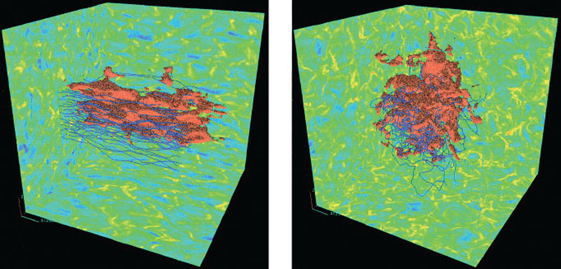Figure 3. Two simulations of driven magnetohydrodynamic turbulence, one with a low Alfvén Mach number (left) and one with a high Alfvén Mach number (right). The colored box walls show the logarithm of density, The blue lines are magnetic field lines. The red surfaces show the distribution of a passive contaminant that has been added to the flow. Reprinted with permission from the AAS from [14].

Third, let us compare the advection term to the viscous term. Taking the ratio of these two gives

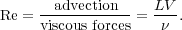(55)

The quantity we have defined is called the Reynolds Number, and it clearly characterizes the importance of viscous forces. If Re >> 1, this means that viscosity is unable to change fluid velocities on a timescale comparable to the natural crossing timescale of the flow. We can also think of the Reynolds number as describing a characteristic size scale L ~ / V on which motions are damped. Motions larger than this scale are unimpeded by viscosity, while smaller scale motions are damped out.

For diffuse gases, the kinematic viscosity = 2 , where is the RMS particle speed and is the mean free path. The former is comparable to the sound speed, ~ 0.2 km s^-1, while the latter is of order the inverse of the cross section times the particle density, ~ 1 / (n ). For a typical molecule size of 1 nm and a density of 100 cm^-2, this gives ~ 10¹² cm. Thus we have ~ 10¹⁶ cm² s^-1, and putting this together with our characteristic size and velocity scales gives Re ~ 10⁹. We therefore learn that molecular cloud flows are extremely non-viscous. An important implication of this is that they are almost certainly turbulent, since essentially all flows with Re 10³ are observed to be turbulent.

Finally, let's apply our non-dimensionalization treatment to the induction equation. Doing so, the two terms on the right hand side are of order

(56)

In analogy with the Reynolds number, we define the ratio of these two terms by the Magnetic Reynolds Number

(57)

The significance of Rm is that, when it is large, the advection term in the induction equation is much larger than the resistive one, and this means that magnetic field is simply carried around by the fluid. We describe this situation as flux-freezing, meaning that lines of magnetic flux passing through a fluid element move with that fluid element at all times.

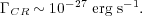
The value of the magnetic Reynolds number depends on the resistivity, which is tricky to calculate. We won't do so in these lectures, but we can outline the main process that contributes to it: ion-neutral drift, also known as ambipolar diffusion. In a molecular cloud, most of the gas is actually neutral, not ionized, and so it doesn't feel magnetic forces. Only the ions do. However, the ions collide with the neutrals, and if those collisions are frequent enough then they will transmit the magnetic force to the neutrals. However, this process isn't perfect. If there are too few ions, then neutrals may go a long time before encountering an ion, and they will begin to drift with respect to the ions, since they ions are being pulled by magnetic forces that the neutrals don't feel. For this reason the resistivity depends on the ionization fraction, with lower ionization fractions giving higher resistivities.

In a molecular cloud the ionization fraction is controlled by the balance between cosmic ray ionizations and recombinations of electrons with ions, and calculations of this process (e.g. [15]) suggest that, at a density of n ~ 100 cm^-3, typical ionization fractions are about 10^-6. That might not seem like much, but it's enough to produce a fairly small resistivity - working through the calculation gives Rm ~ 50 for our typical parameters. We therefore conclude that resistivity is not significant on GMC scales, and flux-freezing holds. However, note that, as with viscosity, we can define a characteristic scale where resistivity does become important, which is L / Rm. This is ~ 0.5 pc, and this means that, on small scales, we expect magnetic fields to begin to decouple from the gas. We'll return to this issue later on.

3.3. The Virial Theorem

As our final topic in this lecture, we will derive a theorem that describes the large-scale behavior of molecular clouds. This is the virial theorem, which is a sort of integrated version of the equations of motion. Like the equations of motion, there is both an Eulerian form and a Lagrangian form of the virial theorem, depending on which version of the equations of motion we start with. We'll derive the Eulerian form here, but the derivation of the Lagrangian form proceeds in a similar manner, and can be found in many standard textbooks. This derivation follows that of McKee & Zweibel [16].

To derive the virial theorem, we begin with the MHD equations of motion, without either viscosity or resistivity (since neither of these are important for GMCs on large scales) but with gravity. We leave in the pressure forces, even though they are small, because they're also trivial to include. Thus we have

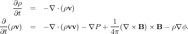(58) (59)

Here is the gravitational potential, so - is the gravitational force per unit volume.

These equations are the Eulerian equations written in conservative form. The first is conservation of mass: it says that the rate of change of density is equal to the flux of mass into or out of a given volume. The second is conservation of momentum: it says that the rate of change of momentum is given by the flux of momentum in or out of a given volume plus the changes in momentum due to gas pressure, magnetic forces, and gravitational forces. Note here that in the second equation the term vv is a tensor - in tensor notation, its elements are v_i v_j.

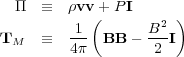
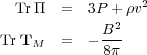
Before we begin, life will be a bit easier if we re-write the entire second equation in a manifestly tensorial form - this simplifies the analysis tremendously. To do so, we define two tensors: the fluid pressure tensor and the Maxwell stress tensor T_M, as follows:

(60) (61)

Here I is the identity tensor. In tensor notation, these are

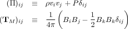(62) (63)

With these definitions, the momentum equation just becomes

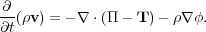(64)

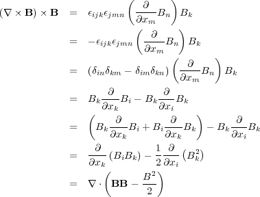
The substitution for is obvious. The equivalence of · T_M to 1 / (4) ( × B) × B is easy to establish with a little vector manipulation, which is most easily done in tensor notation:

(65) (66) (67) (68) (69) (70) (71)

To derive the virial theorem, we begin by imagining a cloud of gas enclosed by some fixed volume V. The surface of this volume is S. We want to know how the overall distribution of mass changes within this volume, so we begin by writing down a quantity the represents the mass distribution. This is the moment of inertia:

(72)

We want to know how this changes in time, so we take its time derivative:

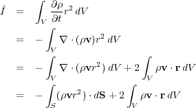(73) (74) (75) (76)

In the first step we used the fact that the volume V does not vary in time to move the time derivative inside the integral. Then in the second step we used the equation of mass conservation to substitute. In the third step we brought the r² term inside the divergence. Finally in the fourth step we used the divergence theorem to replace the volume integral with a surface integral.

Now we take the time derivative again, and multiply by 1/2 for future convenience:

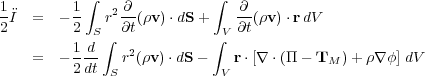(77) (78)

The term involving the tensors is easy to simplify using a handy identity, which applies to an arbitrary tensor. This is a bit easier to follow in tensor notation:

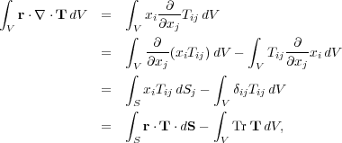(79) (80) (81) (82)

where Tr T = T_ii is the trace of the tensor T.

Applying this to our result our tensors, we note that

(83) (84)

Inserting this result into our expression for give the virial theorem, which I will write in a more suggestive form to make its physical interpretation clearer:

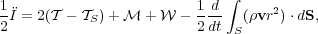(85)

where

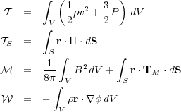(86) (87) (88) (89)

Written this way, we can give a clear interpretation to what these terms mean. is just the total kinetic plus thermal energy of the cloud. _s is the confining pressure on the cloud surface, including both the thermal pressure and the ram pressure of any gas flowing across the surface. is the the difference between the magnetic pressure in the cloud interior, which tries to hold it up, and the magnetic pressure plus magnetic tension at the cloud surface, which try to crush it. is the gravitational energy of the cloud. If there is no external gravitational field, and comes solely from self-gravity, then is just the gravitational binding energy. The final integral represents the rate of change of the momentum flux across the cloud surface.

is the integrated form of the acceleration. For a cloud of fixed shape, it tells us the rate of change of the cloud's expansion of contraction. If it is negative, the terms that are trying to collapse the cloud (the surface pressure, magnetic pressure and tension at the surface, and gravity) are larger, and the cloud accelerates inward. If it is positive, the terms that favor expansion (thermal pressure, ram pressure, and magnetic pressure) are larger, and the cloud accelerates outward. If it is zero, the cloud neither accelerates nor decelerates.

We get a particularly simple form of the virial theorem if there is no gas crossing the cloud surface (so v = 0 at S) and if the magnetic field at the surface to be a uniform value B₀. In this case the virial theorem reduces to

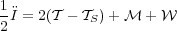(90)

with

(91) (92)

In this case _s just represents the mean radius times pressure at the virial surface, and just represents the total magnetic energy of the cloud minus the magnetic energy of the background field over the same volume.

Notice that, if a cloud is in equilibrium ( = 0) and magnetic and surface forces are negligible, then we have 2 = -, which is what went into our definition of the virial ratio above: _vir = 2 / ||.