


Our main goal in this section is to compare the properties of GMCs made with different telescopes, resolutions, and sensitivities. We use GMC catalogs from the studies of the four galaxies listed above, and we supplement our work with a sample of GMCs in M31 (Rosolowsky, 2006) as well as a compilation of molecular clouds in the outer Milky Way as observed by Dame et al. (2001) and cataloged in Rosolowsky and Leroy (2006).
To aid in the systematic comparison of cloud properties, Rosolowsky and Leroy (2006, hereafter RL06) have recently published a method for minimizing the biases that plague such comparisons. For example, measurement of the cloud radius depends on the sensitivity of the measurements, and RL06 suggest a robust method to extrapolate to the expected radius in the limit of infinite sensitivity. They also suggest a method to correct cloud sizes for beam convolution, which has been ignored in many previous studies of extragalactic clouds. We use the RL06 extrapolated moment method on all of the data used in this paper since it is least affected by relatively poor signal-to-noise and resolution effects. We have also applied the RL06 methodology to the outer Milky Way data of Dame et al. (2001) rather than relying on published properties (e.g., Heyer et al., 2001). It is for this reason that we have not included the cloud properties of Solomon et al. (1987) in our plots, but we do make comparisons to their work at the end of this section. Except where noted, we consider only clouds that are well-resolved by the telescope beam; the GMCs must have angular diameters at least twice that of the beam used to observe them.
Are we seeing single or multiple objects in the beam? The issue of velocity blending of multiple clouds in the beam is much less of an issue in extragalactic observations than in the Galactic case, where the overwhelming majority of GMCs are observed only in the Galactic plane. Extragalactic observations of all but the most highly inclined galaxies do not suffer from this problem and as can be seen in Figs. 1 - 4, the clouds are, in general, spatially well separated, ensuring that we are almost always seeing only a single GMC along the line of sight.
One of the long debated questions related to GMCs is: how does metallicity affect the value of XCO, the conversion factor from CO line strength to H2 column density? Fig. 6 is a plot of the virial mass of the GMCs as a function of CO luminosity. Diagonal lines are lines of constant XCO. A compilation of XCO values is given in Table 2. We note first that most of the points lie above the dashed line that indicates the value determined from gamma-rays in the Milky Way (Strong and Mattox, 1996). A value of XCO = 4× 1020 cm-2 (K km s-1)-1 would allow virial masses to be derived to within about a factor of two for all of the GMCs in our sample, with the clouds in the SMC and the outer Galaxy requiring a somewhat higher value.
 |
Figure 6. Plot of the virial mass of the GMCs in our sample as a function of luminosity. The value of XCO from gamma-ray investigations in the Milky Way (Strong and Mattox, 1996) is shown by the dashed line. The plot shows that while there are some differences in XCO from galaxy to galaxy, except for the SMC, a value of XCO = 4 × 1020 cm-2 (K km s-1)-1 can be used for all of the other galaxies to a reasonable degree of approximation. |
| Galaxy | Mean XCO | Scatter in XCO a |
| × 1020 cm-2 (K km s-1)-1 | × 1020 cm-2 (K km s-1)-1 | |
| SMC | 13.5 ± 2.6 | 2.2 |
| LMC | 5.4 ± 0.5 | 1.7 |
| IC 10 | 2.6 ± 0.5 | 2.2 |
| M33 | 3.0 ± 0.4 | 1.5 |
| M31 | 5.6 ± 1.1 | 2.7 |
| Quad 2 b | 6.6 ± 0.6 | 2.0 |
| Local Group c | 5.4 ± 0.5 | 2.0 |
| a Scatter is a factor based on median absolute
deviation of the log.
b Clouds with luminosities corresponding to
MLum c Excluding Milky Way. |
||
Note, however, that the SMC clouds are systematically higher in this plot than the GMCs for any other galaxy, and that the GMCs in IC 10 are systematically a bit lower. Solving for XCO in the SMC, gives a value of 13.5 × 1020 cm-2 (K km s-1)-1, more than a factor of 3 above the mean. In contrast, IC 10 yields XCO = 2 × 1020 cm-2 (K km s-1)-1. Surprisingly, the galaxies differ in metallicity from one another only by a factor of two, and both are much less than solar. In M33, the metallicity decreases by almost an order of magnitude from the center out (Henry and Howard, 1995), but Rosolowsky et al. (2003) find no change in XCO with radius. Although metallicity may be a factor in determining XCO in different galaxies, there is no clear trend with metallicity alone - other factors appear to be as important as the metallicity in determining XCO.
The discrepancy between the Galactic gamma-ray value of 2 × 1020 cm-2 (K km s-1)-1 and the virial value we derive here is not necessarily a problem. Taken at face value, it may be telling us is that the GMCs are not in virial equilibrium, but are nearly gravitationally neutral: the overall potential energy is equal to the kinetic energy. The gamma-ray value of XCO is independent of the dynamical state of the cloud, thus, uncertainties about the self-gravity of GMCs do not come into play. Since GMCs do not look as if they are in virial equilibrium (they are highly filamentary structures and do not appear to be strongly centrally concentrated), these two different values of XCO are consistent if the clouds are only marginally self-gravitating.
 |
 |
Figure 7. (Left)
Luminosity vs. Line
width plot for all of the resolved clouds in our survey. The dashed
line, LCO
|
|
The left-hand panel of Fig. 7 is a plot of the
CO luminosity of GMCs as a function of line width. It may be thought of
as a plot of H2 mass vs. line width for a single, but
undetermined, value of XCO.
The dashed line, is the relation LCO

 v4,
is not a fit, but is a good representation of the data
for both the five external galaxies in our sample as well as for the
outer Milky Way. The scatter in the relationship is 0.5 dex, or a
factor of 3 over three orders of magnitude in luminosity. If the GMCs
are self-gravitating, then they obey
v4,
is not a fit, but is a good representation of the data
for both the five external galaxies in our sample as well as for the
outer Milky Way. The scatter in the relationship is 0.5 dex, or a
factor of 3 over three orders of magnitude in luminosity. If the GMCs
are self-gravitating, then they obey
 |
(1) |
where  is a constant of
order unity. Provided the CO luminosity is
proportional to the mass of a GMC, the plot shows that
M(H2)
v4;
thus
is a constant of
order unity. Provided the CO luminosity is
proportional to the mass of a GMC, the plot shows that
M(H2)
v4;
thus
 |
(2) |
These two relations are shown on the left- and right-hand sides of Fig. 8 respectively.
 |
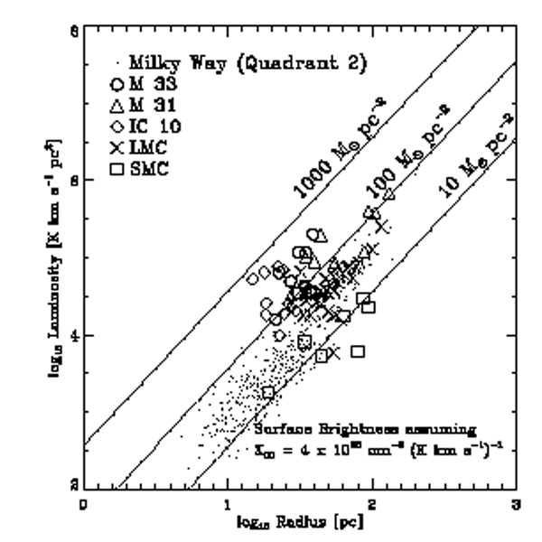 |
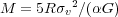
Figure 8. (left) Line width-size relation for the GMCs in our sample. The dashed line is the relation found for the GMCs in the inner Milky Way, showing a clear offset from the extragalactic GMCs. (Right) Luminosity vs. Radius relation for the GMCs in our sample. Solid lines are lines of constant surface density assuming XCO = 4 × 1020 cm-2 (K km s-1)-1. The galaxies show clear differences in CO luminosity for a given cloud radius. |
|
The advantage of a luminosity-line width plot, especially for
extragalactic studies is that one need not resolve the individual
clouds, since the luminosity, and by implication, the mass, is
independent of resolution. One need only be sure that individual GMCs
are isolated in the beam. The right-hand panel in
Fig. 7
shows all of the individual clouds identified in the galaxy surveys,
most of which are unresolved. We see that the clouds populate the
same LCO
v4
line as in the left-hand panel.
This plot demonstrates probably better than any other that the GMCs in
our sample are much more alike than they are different.
The left-hand side of Fig. 8 is the size-line width
relation for the GMCs in our sample. The dashed line is the size-line
width relation for GMCs in the inner region of the Milky Way from
Solomon et al.
(1987).
First, we note that the correlation for the
extragalactic clouds is very weak. However, if we add the outer
Galaxy clouds, the correlation does seem to be consistent with a power
law relation
v
R0.5. However, there is a clear
offset from the relation determined for the inner Galaxy (dashed line,
Solomon et al.,
1987).
At least part of this offset can be attributed
to differences in the methods used to measure cloud properties. The
sense of the offset is that for a given cloud radius, inner Milky Way
clouds have larger line widths. This may be partially due to the
relatively high value of TA used by
Solomon et al.
(1987)
to define the cloud radius, implying that the clouds might be inferred
to be smaller for a given value of
v.
But part of the offset may also be real. We see that there is a clear
separation of the clouds by galaxy in the plot. The IC 10 clouds lie
to the left of the diagram, while the LMC clouds lie to the right.
The SMC clouds tend to lie at the bottom of the
group. The apparently
weak correlation of extragalactic clouds is probably due to the small
dynamic range in the plot compared to the measurement error in the
cloud properties; the rms scatter in Fig. 8
(left) is only 0.2 dex, or less than a factor of two. We therefore conclude
that the GMCs in our sample are consistent with a power law relation
v
R0.5. There are, however, real differences in
the coefficient of proportionality, and this gives rise to some of the
scatter in the relationship. The size-line width relationship arises
from the turbulent nature of the molecular gas motions. Differences
in the constant of proportionality imply variations in the
normalization of the turbulent motions of GMCs in different galaxies,
independent of cloud luminosity.
These conclusions help to explain Fig. 8
(right), which is a plot of luminosity vs. radius. Assuming that
luminosity is proportional to mass, at least within a single galaxy, we
can plot lines of constant surface brightness. After all,
Fig. 6 suggests that the clouds have a constant
surface brightness. In fact, it appears that for a given galaxy, the
individual GMCs are strung out along lines of constant surface density,
but with each galaxy lying on a different line. The SMC clouds, for
example, have a mean surface density of 10
M pc-2, but the
IC 10 clouds have a mean surface density > 100
M
pc-2. A direct interpretation of Fig. 8
(right) implies that for a given radius, the SMC
clouds are less luminous than the rest, and the IC 10 clouds are
more luminous. Another way of saying this is that for a given cloud
luminosity, the SMC clouds are larger, as are the LMC clouds, only less
so. This difference disappears, for the most part, if we consider the
mass surface density rather than the surface brightness. In that case
one must multiply the luminosity of the GMCs in each galaxy by its
appropriate value of XCO. When that is done, the
difference in the mean surface density from galaxy to galaxy is less
than a factor of two.
pc-2, but the
IC 10 clouds have a mean surface density > 100
M
pc-2. A direct interpretation of Fig. 8
(right) implies that for a given radius, the SMC
clouds are less luminous than the rest, and the IC 10 clouds are
more luminous. Another way of saying this is that for a given cloud
luminosity, the SMC clouds are larger, as are the LMC clouds, only less
so. This difference disappears, for the most part, if we consider the
mass surface density rather than the surface brightness. In that case
one must multiply the luminosity of the GMCs in each galaxy by its
appropriate value of XCO. When that is done, the
difference in the mean surface density from galaxy to galaxy is less
than a factor of two.
 |
Figure 9. Cumulative mass distribution for the Galaxies in our sample. The mass distributions have been normalized by the area surveyed in each galaxy. In this figure, we use all clouds above the completeness limits in each survey, whether or not the clouds are resolved. All of the galaxies look similar except for M33 which has a steeper mass spectrum than the others. |
In Fig. 7 we see that the GMCs in the SMC are well-separated
from the GMCs in M31, implying that the median luminosity of the two
sets of clouds is different by nearly two orders of magnitude. The
differences due to XCO are only a factor of about 4;
but is the distribution of GMC masses in the two systems really
different? There are not enough clouds to measure a mass spectrum in the
SMC, but Fig. 9
shows the mass distribution of molecular
clouds normalized to the survey area for the other five galaxies.
Power-law fits to the masses of all cataloged molecular clouds above
the completeness limit give the index of the mass distributions listed
in Table 3. All of the galaxies have remarkably
similar mass distributions except for M33, which is much steeper than
the others. In addition, the mass distributions in M31 and the LMC show a
truncation at high mass similar to that found in the inner Milky Way
(e.g.,
Williams and McKee,
1997)
suggesting that there is a
characteristic cloud mass in these systems. In addition,
Engargiola et al.
(2003)
also argue for a characteristic cloud mass
in M33 but it is not at the high mass end, as it is for
the LMC
and M31; rather it has a value of 4 - 6 ×
104
M.
The variation in the mass distributions is unexplained and
may offer an avenue to understanding differences in star formation
rates between galaxies.
| Galaxy | Index |
| LMC | -1.74 ± 0.08 |
| IC 10 | -1.74 ± 0.41 |
| M33 | -2.49 ± 0.48 |
| M31 | -1.55 ± 0.20 |
| Outer MW | -1.71 ± 0.06 |
 5
× 104
M
5
× 104
M