5. IMPLICATIONS OF PROBABILISTIC MODELLING

We have seen the implications of probabilistic modelling for a low- regime when Monte Carlo simulations (or covolution of the stellar luminosity function) are required. However, we have shown that some characteristics of stochasticity are present independently of (as in SBFs and partial correlations). In addition, we have seen that we can combine different probability distributions to describe new situations, as for integrated luminosities at a given or integrated luminosities of clusters that follow a or age distribution. Let us explore the implications of such results.

5.1. Metrics of fitting

The first implication of the modelling of stellar populations is that the redder the wavelength, the greater is the scatter, since fewer stars contribute to red wavelengths than to blue wavelengths in absolute and relative terms. In fact, each wavelength can fluctuate around the mean of the corresponding distribution of integrated luminosities in a different way, even though it is correlated with the other wavelengths. This naturally implies that for each age and metallicity, each model has its own fitting metrics.

We can take advantage of N_eff or SBF definitions to theoretically define the weight for each wavelength in a ² fit. In fact, a good ² fit cannot be better than the physical dispersion of the model, which is a physical limit. Exceedance of this physical limit (overfitting) leads to a more precise but erroneous result. Fig. 9, taken from Cerviño and Luridiana (2009), illustrates the physical dispersion used to identify overfitting for SBFs.

Figure 9. Top: Integrated mean spectra of a 1-Gyr-old cluster. Bottom: 1 and 2 confidence intervals for the mean-averaged dispersion (L - µ1;N'(L) / √(µ1;N'(L)). Figure from Cerviño and Luridiana (2009).

An additional advantage of including the physical weight in the fit is that it breaks degeneracies that are present when observational data are fitted only to the mean value for parametric models. For instance, Fig. 10, taken from Buzzoni (2005), illustrates breaking of age-metallicity degeneracy using N_eff. Given that the allowed scatter depends on age and metallicity, the resulting ² defines the probability that a fit will produce different results.

Figure 10. Theoretical spectral energy distribution (upper plots) and effective stellar contributors (Neff) (lower plots) for two SSPs from population synthesis models described by Buzzoni (1989, 1993) in the spectral region of the MgII and MgI features around 2800 Å. The models refer to a 2-Gyr SSP with red HB morphology and a 15-Gyr population with blue HB, as labelled. In spite of the close similarity of the spectra, the two SSPs display a large difference in terms of Neff, and hence there is much greater statistical scatter in the spectral features expected for the older SSP. Figure from Buzzoni (2005).

An unexplored area involves taking full advantage of (L_i, L_j), which can be obtained theoretically. In fact, the covariance coefficients and variance define a covariance matrix that can be directly implemented in a ² fit. However, as far as I know, computation of (L_i, L_j) has not been implemented and is not considered in any synthesis code (exceptions are Cerviño et al. 2001, Cerviño et al. 2002, Cerviño and Valls-Gabaud 2003, González et al. 2004) but they use a Poisson approximation of the stellar luminosity function and the covariance coefficients obtained are not correct).

5.2. The population and the sample definition

The second implication is related to the definition of the population described by computed distributions. We have seen that we can define populations composed of = 1 stars, which are CMD diagrams, and that we can analyse such populations as long as we have enough events n_sam to describe the distribution.

We can also define populations composed of events with a similar number of stars, , taking advantage of additional information about the source. For instance, we can take the luminosity profile of a galaxy. We can assume that for a given radius, the number of stars is roughly the same (additional information in the form of the geometry of the galaxy is required). Hence, we can evaluate the scatter for the assumed profile, which, independent of observational errors, must be wavelength-dependent. At each galactocentric radius, we are sampling different (L₁... L_n) distributions with different n_sam elements. It is even possible that in the outer parts, where is lower, we find pixels forming a binomial or extremely asymmetric distribution. However, the better our sampling of such distributions, the better will be our characterisation of the population parameters at this radius. Finally, our results for stellar populations must be independent of the radius range chosen once corrected for the radial profile (see Cerviño et al. 2008 for details on such corrections). Hence, we can perform a cross-validation of our results by repeating the analysis by integration over large radial ranges; this means that we reduce n_sam and increase . The only requirements are: (1) must be kept constant in each of the elements of the sample ; and (2) sufficient n_sam elements are required for correct evaluation of the variance (c.f. Eq. (10)). The results obtained must also be consistent with the stellar population obtained using the integral light for the whole galaxy. Note that if we use SBF we do not need to know the value of , but just need to ensure that it is constant (but unknown) in the n_sam elements used.

A similar study can be performed using different ways to divide the image. For example, we can take slices of a spherical system and use each slice to compute the variance of the distribution (see Buzzoni 2005 for an example). A similar technique can be applied to IFU observations. The problem is to obtain n_sam elements with a similar number of stars and stellar populations that allow us to estimate the scatter (SBF) for comparison with model results. In summary, we can include additional information about the system (geometry, light profile, etc.) in inferences about the stellar populations.

Finally, we can modify the (L₁... L_n) distributions to include other distributions representing different objects. For instance, the globular cluster distribution of a galaxy (assuming they have the same age and metallicity, in agreement with Yoon et al. 2006) implicitly includes a distribution of possible values. Since these globular clusters have intrinsically low values, it is possible that some clusters will be in the biased regime described in Fig. 7. Since the few clusters dominated by PMS stars are luminous, they will be observed and will be extremely red in colour, even redder than the mean colour of parametric models (Fig. 8). In addition, there would be a blue tail corresponding to faint clusters with low comprising mainly clusters with low-mass MS stars (see Cerviño and Luridiana 2004 for more details).

5.3. Some rules of thumb

I finish this section with some rules of thumb that can be extracted from the modelling of stellar populations when applied to the inference of physical properties of stellar systems.

First, the relevant quantity in describing possible luminosities is not the total mass of the system, but the total mass (or number of stars) observed for your resolution elements, . The other relevant quantity is the number of resolution elements n_sam for a given . The lower the ratio of to n_sam, the better. In the limit, the optimal case is a CMD analysis.

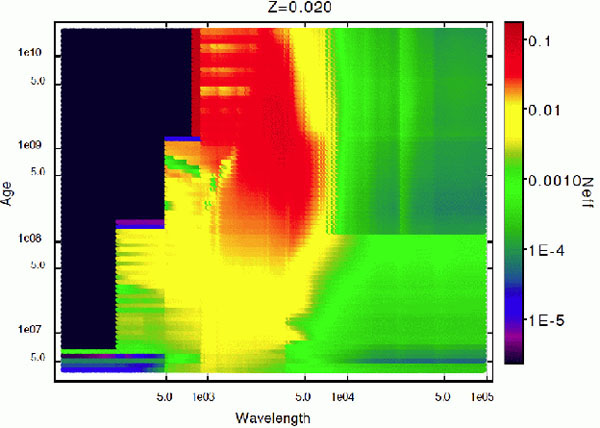
Second, the scatter depends not only on but also on the age and wavelength considered. Fig. 11 shows N_eff values for SSP models with metallicity Z = 0.020 for different ages and wavelengths. As I showed earlier, the lower N_eff is, the greater is the scatter. Fig. 11 shows that blue optical wavelengths with < 5000 Å have intrinsically lower scatter than red wavelengths, independent of . The range 5000-8000 Å has intermediate scatter and scatter increases for wavelengths longer than ~ 8000 Å, depending on the age. In comparison to age determinations that do not consider intrinsic dispersion (i.e. all wavelengths have a similar weight), the safest age inferences correspond to ages between 8 and ~ 200 Myr since variation of N_eff values with wavelength is lower in this mass range.

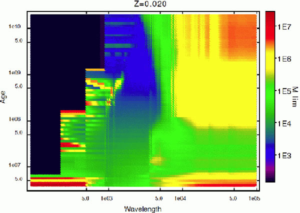Figure 11. Summary of Neff values (left) and mean total mass Mlim for 1, ≤ 0.1 (right) as a function of L age and L wavelength for Z = 0.020 SSP models.

Fig. 11 also shows the mean total mass for _1, ≤ 0.1 as a function of age and wavelength for Z = 0.020 SSP models. This is a quantitative visualization of how the average total mass needed to reach a Gaussian-like regime varies with age and wavelength. It is evident that blue optical wavelengths reach a Gaussian regime at a lower average total mass when compared to other wavelengths. In contrast, red wavelengths not only have greater scatter, but this scatter is also associated with non-Gaussian distributions for a wider range of average total mass. Thus, we can strengthen the statement about age inferences: the safest age inferences correspond to ages between 8 and ~ 200 Myr if the cluster mass is greater than 10⁵ M.

Third, the input distributions (m₀, t, Z) or IMF and SFH define the output distributions. It should be possible to obtain better fits (more precise, but not necessarily more accurate) by changing the input distributions. However, we must be aware that we have explored the possible output distributions before any such changes.

For instance, low-mass clusters have strong fluctuations around the IMF; each cluster (each IMF realization) could produce an excess or deficit of massive stars. Using the mean value obtained by parametric models, a top-heavy or bottom-heavy IMF would produce a better fit of models and data. Such IMF variations would undoubtedly be linked to variations in age and the total mass/number of stars for a system. However, Monte Carlo simulations can also produce a better fit without invoking any IMF variation. It is possible that Monte Carlo simulations using distributions of different IMFs (e.g. combining IMFs with a variable lower or upper mass limit with a distribution of possible lower or upper mass limits) would produce even better fits. I am sure that the approach using only the mean value is methodologically erroneous. However, it is not clear which of the two solutions obtained by Monte Carlo simulations is the best unless one of the hypotheses (fixed IMF or a distribution combining different IMFs) is incompatible with observational data.

As a practical rule, before exploring or claiming variations in the input parameters, a check is required to ensure that such input parameters are actually incompatible with observational data.

Another issue is how to evaluate scatter outside the SSP hypothesis. Formally, we may consider any SFH as a combination of SSPs. Hence, for any SFH scenario evaluated at time t_mod, we can assume that the scatter can be evaluated using the most restrictive SSP situation in the time range from 0 to t_mod. For instance, Fig. 11 shows that the ionising flux ( ≲ 912 Å) requires an average total mass greater than 10⁵ M to reach a Gaussian-like regime. Hence, we must ensure that at least 10⁵ M has been formed in each SSP comprising the SFH. Assume that 1 Myr is the time interval used to define a star formation rate. This implies that there would be no Gaussian-like distributions for SFR less than 0.1 M year^-1 (i.e. there would be a bias in the inferences obtained using the mean obtained by parametric models). However, a more quantitative study of this subject is required. da Silva et al. (2012) have suggested additional ideas on the evaluation of scatter including the SFH.

Fourth, regarding the output parameters and inferences for time and the total mass/number of stars, we can summarize the following rules:

1. Use all available information for the system, including previous inferences. However, wavelength ranges used for inferences in the literature must be considered. Additional criteria, such as those in the following points, can be used to evaluate roughly which inferences are more reliable.

   Additional information on the system can be obtained from images and other data that, although not used directly in the inferences, constrain the possible range of solutions. Recovery of a complete picture of the system compatible with all the available information should be the aim, and not just a partial picture that can be drawn from particular data.

   It is particularly useful to look for the `smoking guns' for age inference: for example, emission lines in star-forming systems imply an age less than 10 Myr ; Wolf-Rayet stars imply an age less than 6 Myr (neglecting binary systems); supernova emission or supernova remnants (from optical, radio or X-ray observations) imply an age less than 50 Myr; high-mass X-ray binaries imply previous supernova events, and hence an age greater than 3 Myr. For instance, Fouesneau et al. (2012) showed that the use of broad-band photometry with narrow-band H<sub>α</sub> photometry greatly improves the quality of inferences. However, note that the presence of a `smoking gun' helps to define age ranges, but the absence of smoking guns does not provide information if the mass/number of stars in observations is not known.

2. Always obtain an estimate of the mass/number of stars in the resolution element. The confidence of an age inference cannot be evaluated unless an estimate of the mass/number of stars of such an age has been obtained (see Popescu and Hanson 2010b for additional implications of this point).

3. Identify the integrated luminosity distribution regime for the system considered . ² fitting including the physical variance and covariance coefficients is optimal for the Gaussian regime, but it fails for other distributions. Fig. 11 can be used to identify Gaussianity. For large wavelength coverage, for which different regimes would be present, rejection of some parts of the spectra in the fit can be considered; it is better to obtain a less precise but more accurate result than a very precise but erroneous result caused by overfitting; in any case, such information can be used as a guide to obtain a complete picture of the system.

4. When using diagnostic diagrams (indices), compare the location of the parametric model, individual stars and observations. It is especially useful to identify the origin of outliers in diagnostic diagrams, and to evaluate the expected range of scatter in the model.
5. In general, CMDs analyses are more robust than analyses of integrated spectra. If such information is available, use it and do not try surpass CMDs, which is simply impossible. The sum of (unknown) elements in a sample cannot provide more information than knowledge for all the particular elements of the sample.
6. Blue wavelengths (3000-5000 Å) are robust. We have shown that blue wavelengths have intrinciscally lower physical scatter than any other wavelengths. Hence, when comparing different inferences in the literature, those based on just blue wavelengths are the most accurate. They may not be the most precise, but blue wavelengths always provide better fitting than any other wavelength. Hence, take the greatest possible advantage of blue wavelengths (e.g. when using normalized spectra to a given wavelength to obtain SFH, use blue wavelengths).
7. A good solution is the distribution of possible solutions. I discussed this in Section 5.1, but I would like to emphasise the point. The best ² value would be a numerical artefact (e.g. local numerical fluctuations). For instance, it seems surprising that codes that infer the SFH using the mean value of parametric models do not usually quote any age-metallicity degeneracy, although it is present at a spectral level (c.f. Fig. 10). In fact, it is an artefact of using only the best ² fit when results are presented. Again, I refer to Fouesneau et al. (2012) as an example of how the use of the distribution of possible solutions improve inferences.