2. OBSERVED PROPERTIES OF GMCs

2.1. GMCs and Star Formation

Molecular gas is strongly correlated with star formation on scales from entire galaxies (Kennicutt 1989, Kennicutt 1998, Gao and Solomon 2004, Saintonge et al. 2011a) to kpc and sub-kpc regions (Wong and Blitz 2002, Bigiel et al. 2008, Rahman et al. 2012, Leroy et al. 2013) to individual GMCs (Evans et al. 2009, Heiderman et al. 2010, Lada et al. 2010, Lada et al. 2012). These relations take on different shapes at different scales. Early studies of whole galaxies found a power-law correlation between total gas content (H i plus H₂) and star formation rate (SFR) with an index N ~ 1.5 (Kennicutt 1989, Kennicutt 1998). These studies include galaxies that span a very large range of properties, from dwarfs to ultraluminous IR galaxies, so it is possible that the physical underpinnings of this relation are different in different regimes. Transitions with higher critical densities such as HCN(1-0) and higher-J CO lines (Gao and Solomon 2004, Bayet et al. 2009, Juneau et al. 2009, García-Burillo et al. 2012) also show power-law correlations but with smaller indices; the index appears to depend mostly on the line critical density, a result that can be explained through models (Krumholz and Thompson 2007, Narayanan et al. 2008b, Narayanan et al. 2008a).

Within galaxies the star formation rate surface density, _SFR, is strongly correlated with the surface density of molecular gas as traced by CO emission and only very weakly, if at all, related to atomic gas. The strong correlation with H₂ persists even in regions where atomic gas dominates the mass budget (Schruba et al. 2011, Bolatto et al. 2011). The precise form of the SFR-H₂ correlation is a subject of study, with results spanning the range from super-linear (Kennicutt et al. 2007, Liu et al. 2011, Calzetti et al. 2012) to approximately linear (Bigiel et al. 2008, Blanc et al. 2009, Rahman et al. 2012, Leroy et al. 2013) to sub-linear (Shetty et al. 2013). Because CO is used to trace H₂, the correlation can be altered by systematic variations in the CO to H₂ conversion factor, an effect that may flatten the observed relation compared to the true one (Shetty et al. 2011, Narayanan et al. 2011, Narayanan et al. 2012).

The SFR-H₂ correlation defines a molecular depletion time, _dep(H₂) = M(H₂) / SFR, which is the time required to consume all the H₂ at the current SFR. A linear SFR-H₂ correlation implies a constant _dep(H₂), while super-linear (sub-linear) relations yield a time scale _dep(H₂) that decreases (increases) with surface density. In regions where CO emission is present, the mean depletion time over kpc scales is _dep(H₂) = 2.2 Gyr with ± 0.3 dex scatter, with some dependence on the local conditions (Leroy et al. 2013). Saintonge et al. (2011) find that, for entire galaxies, _dep(H₂) decreases by a factor of ~ 3 over two orders of magnitude increase in the SFR surface. Leroy et al. (2013) show that the kpc-scale measurements within galaxies are consistent with this trend, but that _dep(H₂) also correlates with the dust-to-gas ratio. For normal galaxies, using a CO-to-H₂ conversion factor that depends on the local dust-to-gas ratio removes most of the variation in _dep(H₂).

On scales of a few hundred parsecs, the scatter in _dep(H₂) rises significantly (e.g., Schruba et al. 2010, Onodera et al. 2010) and the SFR-H₂ correlation breaks down. This is partially a manifestation of the large dispersion in SFR per unit mass in individual GMCs (Lada et al. 2010), but it is also a consequence of the time scales involved (Kawamura et al. 2009, Kim et al. 2013). Technical issues concerning the interpretation of the tracers also become important on the small scales (Calzetti et al. 2012).

On sub-GMC scales there are strong correlations between star formation and extinction, column density, and volume density. The correlation with volume density is very close to that observed in ultraluminous IR galaxies (Wu et al. 2005). Some authors have interpreted these data as implying that star formation only begins above a threshold column density of _H2 ~ 110-130 M yr^-1 or volume density n ~ 10^4-5 cm^-3 (Evans et al. 2009, Heiderman et al. 2010, Lada et al. 2010, Lada et al. 2012). However, others argue that the data are equally consistent with a smooth rise in SFR with volume or surface density, without any particular threshold value (Krumholz and Tan 2007, Narayanan et al. 2008b, Narayanan et al. 2008a, Gutermuth et al. 2011, Krumholz et al. 2012, Burkert and Hartmann 2013).

2.2. GMCs as a Component of the Interstellar Medium

Molecular clouds are the densest, coldest, highest column density, highest extinction component of the interstellar medium. Their masses are dominated by molecular gas (H₂), with a secondary contribution from He (~ 26%), and a varying contribution from H i in a cold envelope (e.g., Fukui and Kawamura 2010) and interclump gas detectable by H i self-absorption (Goldsmith and Li 2005). Most of the molecular mass in galaxies is in the form of molecular clouds, with the possible exception of galaxies with gas surface densities substantially higher than that of the Milky Way, where a substantial diffuse H₂ component exists (Papadopoulos et al. 2012b, Papadopoulos et al. 2012a, Pety et al. 2013, Colombo et al. 2013).

Molecular cloud masses range from ~ 10² M for small clouds at high Galactic latitudes (e.g., Magnani et al. 1985) and in the outer disk of the Milky Way (e.g., Brand and Wouterloot 1995, Heyer et al. 2001) up to giant ~ 10⁷ M clouds in the central molecular zone of the Galaxy (Oka et al. 2001). The measured mass spectrum of GMCs (see Section 2.3) implies that most of the molecular mass resides in the largest GMCs. Bulk densities of clouds are log[n_H2 / cm^-3] = 2.6 ± 0.3 (Solomon et al. 1987, Roman Duval et al. 2010), but clouds have inhomogenous density distributions with large contrasts (Stutzki et al. 1988). The ratio of molecular to stellar mass in galaxies shows a strong trend with galaxy color from high in blue galaxies (10% for NUV - r ~ 2) to low in red galaxies ( 0.16% for NUV - r 5) (Saintonge et al. 2011a). The typical molecular to atomic ratio in galaxies where both H i and H₂ are detected is R_mol ≡ M_H2 /M_HI ≈ 0.3 with scatter of ± 0.4 dex. The large scatter reflects the fact that the atomic and molecular masses are only weakly correlated, and in contrast with the molecular gas to stellar mass fraction, the ratio R_mol shows only weak correlations with galaxy properties such as color (Leroy et al. 2005, Saintonge et al. 2011a).

In terms of their respective spatial distributions, in spiral galaxies H₂ is reasonably well described by an exponential profile with a scale length ℓ_CO ≈ 0.2 R₂₅, rather smaller than the optical emission (Young et al. 1995, Regan et al. 2001, Leroy et al. 2009, Schruba et al. 2011), where R₂₅ is the 25th magnitude isophotal radius for the stellar light distribution. In contrast, H i shows a nearly flat distribution with typical maximum surface density _HI,max ~ 12 M pc^-2 (similar to the H i column seen toward Solar neighborhood clouds, Lee et al. 2012). Galaxy centers are the regions that show the most variability and the largest departures from these trends (Regan et al. 2001, Bigiel and Blitz 2012). At low metallicities the H i surface density can be much larger, possibly scaling as _HI,max ~ Z^-1 (Fumagalli et al. 2010, Bolatto et al. 2011, Wong et al. 2013). In spiral galaxies the transition between the atomic- and molecular-dominated regions occurs at R ~ 0.4 R₂₅ (e.g., Leroy et al. 2008). The CO emission also shows much more structure than the H i on the small scales (Leroy et al. 2013). In spirals with well defined arms (NGC 6946, M 51, NGC 628) the interarm regions contain at least 30% of the measured CO luminosity (Foyle et al. 2010), but at fixed total gas surface density R_mol is very similar for arm and interarm regions, suggesting that arms act mostly to collect gas rather to directly trigger H₂ formation (Foyle et al. 2010) (see Figure 1). We discuss the relationship between H i and H₂ in more detail in Section 3.3.

Figure 1. (left) CO J = 1-0 image of M 51 from Koda et al. (2009) showing the largest cloud complexes are distributed in spiral arms, while smaller GMCs lie both in and between spiral features. (right) 3 color image of CO J = 1-0 emission from the Taurus molecular cloud from Narayanan et al. (2008c) illustrating complex gas motions within clouds. Colors represents the CO integrated intensities over VLSR intervals 0-5 (blue), 5-7.5 (green) and 7.5-12 (red) km s-1.

2.3. Statistical Properties of GMCs

Statistical descriptions of GMC properties have provided insight into the processes that govern their formation and evolution since large surveys first became possible in the 1980s (see Section 1). While contemporary observations are more sensitive and feature better angular resolution and sampling than earlier surveys, identification of clouds within position-position-velocity (PPV) data cubes remains a significant problem. In practice, one defines a cloud as a set of contiguous voxels in a PPV data cube of CO emission above a surface brightness threshold. Once a cloud is defined, one can compute global properties such as size, velocity dispersion, and luminosity (Williams et al. 1994, Rosolowsky and Leroy 2006). While these algorithms have been widely applied, their reliability and completeness are difficult to evaluate (Ballesteros-Paredes and Mac Low 2002, 2009Pineda et al., 2009bKainulainen et al.), particularly for surveys of ¹²CO and ¹³CO in the Galactic Plane that are subject to blending of emission from unrelated clouds. The improved resolution of modern surveys helps reduce these problems, but higher surface brightness thresholds are required to separate a feature in velocity-crowded regions. High resolution can also complicate the accounting, as the algorithms may identify cloud substructure as distinct clouds. Moreover, even once a cloud is identified, deriving masses and mass-related quantities from observed CO emission generally requires application of the CO-to-H₂ conversion factor or the H₂ to ¹³CO abundance ratio, both of which can vary within and between clouds in response to local conditions of UV irradiance, density, temperature, and metallicity (Bolatto et al. 2013, Ripple et al. 2013). Millimeter wave interferometers can resolve large GMC complexes in nearby galaxies but must also account for missing flux from an extended component of emission.

Despite these observational difficulties, there are some robust results. Over the mass range M > 10⁴ M where it can be measured reliably, the cloud mass spectrum is well-fit by a powerlaw dN/dM ~ M^- (cumulative distribution function N(> M) ~ M^-+1), with values < 2 indicating that most of the mass is in large clouds. For GMCs in the Milky Way, is consistently found to be in the range 1.5 to 1.8 (Solomon et al. 1987, Kramer et al. 1998, Heyer et al. 2001, Roman Duval et al. 2010) with the higher value likely biased by the inclusion of cloud fragments identified as distinct clouds. GMCs in the Magellanic Clouds exhibit a steeper mass function overall and specifically for massive clouds (Fukui et al. 2008, Wong et al. 2011). In M 33, ranges from 1.6 in the inner regions to 2.3 at larger radii (Rosolowsky and Blitz 2005, Gratier et al. 2012).

In addition to clouds' masses, we can measure their sizes and thus their surface densities. The Solomon et al. (1987) catalog of inner Milky Way GMCs, updated to the current Galactic distance scale, shows a distribution of GMCs surface densities _GMC ≈ 150_-70⁺⁹⁵ Mpc^-2 (± 1 interval) assuming a fixed CO-to-H₂ conversion factor X_CO = 2 × 10²⁰ cm^-2 (K km s^-1)^-1, and including the He mass (Bolatto et al. 2013). Heyer et al. (2009) re-observed these clouds in ¹³CO and found _GMC ~ 40 M pc^-2 over the same cloud areas, but concluded that this is likely at least a factor of 2 too low due to non-LTE and optical depth effects. Heiderman et al. (2010) find that ¹³CO can lead to a factor of 5 underestimate. A reanalysis by Roman Duval et al. (2010) shows _GMC ~ 144 M pc^-2 using the ¹³CO rather than the ¹²CO contour to define the area. Measurements of surface densities in extragalactic GMCs remain challenging, but with the advent of ALMA the field is likely to evolve quickly. For a sample of nearby galaxies, many of them dwarfs, Bolatto et al. (2008) find _GMC ≈ 85 M pc^-2. Other recent extragalactic surveys find roughly comparable results, _GMC ~ 40-170 M pc^-2 (Rebolledo et al. 2012, Donovan Meyer et al. 2013).

GMC surface densities may prove to be a function of environment. The PAWS survey of M 51 finds a progression in surface density (Colombo et al. 2013), from clouds in the center (_GMC ~ 210 M pc^-2), to clouds in arms (_GMC ~ 185 M pc^-2), to those in interarm regions (_GMC ~ 140 M pc^-2). Fukui et al. (2008), Bolatto et al. (2008), and Hughes et al. (2010) find that GMCs in the Magellanic Clouds have lower surface densities than those in the inner Milky Way (_GMC ~ 50 M pc^-2). Because of the presence of extended H₂ envelopes at low metallicities (Section 2.6), however, this may underestimate their true molecular surface density (e.g., Leroy et al. 2009). Even more extreme variations in _GMC are observed near the Galactic Center and in more extreme starburst environments (see Section 2.7).

In addition to studying the mean surface density of GMCs, observations within the Galaxy can also probe the distribution of surface densities within GMCs. For a sample of Solar neighborhood clouds, Kainulainen et al. (2009a) use infrared extinction measurements to determine that PDFs of column densities are lognormal from 0.5 < A_V < 5 (roughly 10-100 M pc^-2), with a power-law tail at high column densities in actively star-forming clouds. Column density images derived from dust emission also find such excursions (Schneider et al. 2012, Schneider et al. 2013). Lombardi et al. (2010), also using infrared extinction techniques, find that, although GMCs contain a wide range of column densities, the mass M and area A contained within a specified extinction threshold nevertheless obey the Larson (1981) M ∝ A relation, which implies constant column density.

Finally, we warn that all column density measurements are subject to a potential bias. GMCs are identified as contiguous areas with surface brightness values or extinctions above a threshold typically set by the sensitivity of the data. Therefore, pixels at or just above this threshold comprise most of the area of the defined cloud and the measured cloud surface density is likely biased towards the column density associated with this threshold limit. Note that there is also a statistical difference between "mass-weighed" and "area-weighed" _GMC. The former is the average surface density that contributes most of the mass, while the latter represents a typical surface density over most of the cloud extent. Area-weighed _GMC tend to be lower, and although perhaps less interesting from the viewpoint of star formation, they are also easier to obtain from observations.

In addition to mass and area, velocity dispersion is the third quantity that we can measure for a large sample of clouds. It provides a coarse assessment of the complex motions in GMCs as illustrated in Figure 1. Larson (1981) identified scaling relationships between velocity dispersion and cloud size suggestive of a turbulent velocity spectrum, and a constant surface density for clouds. Using more sensitive surveys of GMCs, Heyer et al. (2009) found a scaling relation that extends the Larson relationships such that the one-dimensional velocity dispersion _v depends on the physical radius, R, and the column density _GMC, as shown in Figure 2. The points follow the expression,

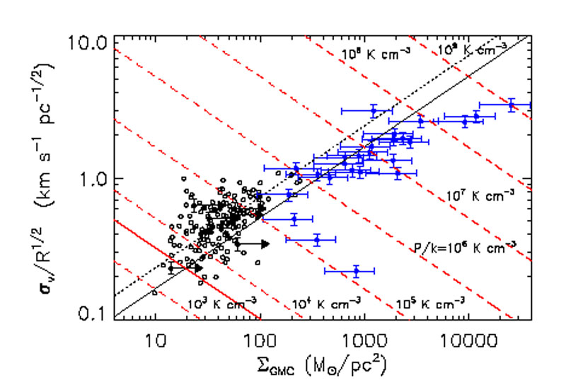Figure 2. The variation of v / R1/2 with surface density, GMC, for Milky Way GMCs from Heyer et al. (2009) (open circles) and massive cores from Gibson et al. (2009) (blue points). For clarity, a limited number of error bars are displayed for the GMCs. The horizontal error bars for the GMCs convey lower limits to the mass surface density derived from 13CO. The vertical error bars for both data sets reflect a 20% uncertainty in the kinematic distances. The horizontal error bars for the massive cores assume a 50% error in the C18O and N2H+ abundances used to derive mass. The solid and dotted black lines show loci corresponding to gravitationally bound and marginally bound clouds respectively. Lines of constant turbulent pressure are illustrated by the red dashed lines. The mean thermal pressure of the local ISM is shown as the red solid line.

More recent compilations of GMCs in the Milky Way (Roman Duval et al. 2010) have confirmed this result, and studies of Local Group galaxies (Bolatto et al. 2008, Wong et al. 2011) have shown that it applies to GMCs outside the Milky Way as well. Equation 1 is a natural consequence of gravity playing an important role in setting the characteristic velocity scale in clouds, either through collapse (Ballesteros-Paredes et al. 2011b) or virial equilibrium (Heyer et al. 2009). Unfortunately one expects only factor of √2 differences in velocity dispersion between clouds that are in free-fall collapse or in virial equilibrium (Ballesteros-Paredes et al. 2011b) making it extremely difficult to distinguish between these possibilities using observed scaling relations. Concerning the possibility of pressure-confined but mildly self-gravitating clouds (Field et al. 2011), Figure 2 shows that the turbulent pressures, P = _v², in observed GMCs are generally larger than the mean thermal pressure of the diffuse ISM (Jenkins and Tripp 2011) so these structures must be confined by self-gravity.

As with column density, observations within the Galaxy can also probe internal velocity structure. Brunt (2003), Heyer and Brunt (2004), and Brunt et al. (2009) used principal components analysis of GMC velocity fields to investigate the scales on which turbulence in molecular clouds could be driven. They found no break in the velocity dispersion-size relation, and reported that the second principle component has a "dipole-like" structure. Both features suggest that the dominant processes driving GMC velocity structure must operate on scales comparable to or larger than single clouds.

2.4. Dimensionless Numbers: Virial Parameter and Mass to Flux Ratio

The virial theorem describes the large-scale dynamics of gas in GMCs, so ratios of the various terms that appear in it are a useful guide to what forces are important in GMC evolution. Two of these ratios are the virial parameter, which evaluates the importance of internal pressure and bulk motion relative to gravity, and the dimensionless mass to flux ratio, which describes the importance of magnetic fields compared to gravity. Note, however, that neither of these ratios accounts for potentially-important surface terms (e.g., Ballesteros-Paredes et al. 1999).

The virial parameter is defined as _G = M_virial / M_GMC, where M_virial = 5_v² R / G and M_GMC is the luminous mass of the cloud. For a cloud of uniform density with negligible surface pressure and magnetic support, _G = 1 corresponds to virial equilibrium and _G = 2 to being marginally gravitationally bound, although in reality _G > 1 does not strictly imply expansion, nor does _G <1 strictly imply contraction (Ballesteros-Paredes 2006). Surveys of the Galactic Plane and nearby galaxies using ¹²CO emission to identify clouds find an excellent, near-linear correlation between M_virial and the CO luminosity, L_CO, with a coefficient implying that (for reasonable CO-to-H₂ conversion factors) the typical cloud virial parameter is unity (Solomon et al. 1987, Fukui et al. 2008, Bolatto et al. 2008, Wong et al. 2011). Virial parameters for clouds exhibit a range of values from _G ~ 0.1 to _G ~ 10, but typically _G is indeed ~ 1. Heyer et al. (2009) reanalyzed the Solomon et al. (1987) GMC sample using ¹³CO J = 1-0 emission to derive cloud mass and found a median _G = 1.9. This value is still consistent with a median _G = 1, since excitation and abundance variations in the survey lead to systematic underestimates of M_GMC. A cloud catalog generated directly from the ¹³CO emission of the BU-FCRAO Galactic Ring Survey resulted in a median _G = 0.5 (Roman Duval et al. 2010). Previous surveys (Dobashi et al. 1996, Yonekura et al. 1997, Heyer et al. 2001) tended to find higher _G for low mass clouds, possibly a consequence of earlier cloud-finding algorithms preferentially decomposing single GMCs into smaller fragments (Bertoldi and McKee 1992).

The importance of magnetic forces is characterized by the ratio M_GMC / M_cr, where M_cr = / (4² G)^1/2 and is the magnetic flux threading the cloud (Mouschovias and Spitzer 1976, Nakano 1978). If M_GMC / M_cr > 1 (the supercritical case) then the magnetic field is incapable of providing the requisite force to balance self-gravity, while if M_GMC / M_cr<1 (the subcritical case) the cloud can be supported against self-gravity by the magnetic field. Initially subcritical volumes can become supercritical through ambipolar diffusion (Mouschovias 1987, Lizano and Shu 1989). Evaluating whether a cloud is sub- or supercritical is challenging. Zeeman measurements of the OH and CN lines offer a direct measurement of the line of sight component of the magnetic field at densities ~ 10³ and ~ 10⁵ cm^-3, respectively, but statistical corrections are required to account for projection effects for both the field and the column density distribution. Crutcher (2012) provides a review of techniques and observational results, and report a mean value M_GMC / M_cr ≈ 2-3, implying that clouds are generally supercritical, though not by a large margin.

2.5. GMC Lifetimes

The natural time unit for GMCs is the free-fall time, which for a medium of density is given by _ff = [3 / (32 G )]^1/2 = 3.4 (100 / n_H2)^1/2 Myr, where n_H2 is the number density of H₂ molecules, and the mass per H₂ molecule is 3.9 × 10^-24 g for a fully molecular gas of cosmological composition. This is the timescale on which an object that experiences no significant forces other than its own gravity will collapse to a singularity. For an object with _G ≈ 1, the crossing timescale is _cr = R / ≈ 2_ff. It is of great interest how these natural timescales compare to cloud lifetimes and depletion times.

Scoville et al. (1979) argue that GMCs in the Milky Way are very long-lived (> 10⁸ yr) based on the detection of molecular clouds in interarm regions, and Koda et al. (2009) apply similar arguments to the H₂-rich galaxy M 51. They find that, while the largest GMC complexes reside within the arms, smaller (< 10⁴ M) clouds are found in the interarm regions, and the molecular fraction is large (> 75%) throughout the central 8 kpc (see also Foyle et al. 2010). This suggests that massive GMCs are rapidly built-up in the arms from smaller, pre-existing clouds that survive the transit between spiral arms. The massive GMCs fragment into the smaller clouds upon exiting the arms, but have column densities high enough to remain molecular (see Section 3.4). Since the time between spiral arm passages is ~ 100 Myr, this implies a similar cloud lifetime _life 100 Myr ≫ _ff. Note, however, this is an argument for the mean lifetime of a H₂ molecule, not necessarily for a single cloud. Furthermore, these arguments do not apply to H₂-poor galaxies like the LMC and M 33.

Kawamura et al. (2009) (see also Fukui et al. 1999, Gratier et al. 2012) use the NANTEN Survey of ¹²CO J = 1-0 emission from the LMC, which is complete for clouds with mass >5 × 10⁴ M, to identify three distinct cloud types that are linked to specific phases of cloud evolution. Type I clouds are devoid of massive star formation and represent the earliest phase. Type II clouds contain compact H ii regions, signaling the onset of massive star formation. Type III clouds, the final stage, harbor developed stellar clusters and H ii regions. The number counts of cloud types indicate the relative lifetimes of each stage, and age-dating the star clusters found in type III clouds then makes it possible to assign absolute durations of 6, 13, and 7 Myrs for Types I, II, and III respectively. Thus the cumulative GMC lifetime is _life ~ 25 Myrs. This is still substantially greater than _ff, but by less so than in M 51.

While lifetime estimates in external galaxies are possible only for large clouds, in the Solar Neighborhood it is possible to study much smaller clouds, and to do so using timescales derived from the positions of individual stars on the HR diagram. Elmegreen (2000), Hartmann et al. (2001) and Ballesteros-Paredes and Hartmann (2007), examining a sample of Solar Neighborhood GMCs, note that their HR diagrams are generally devoid of post T-Tauri stars with ages of ~ 10 Myr or more, suggesting this as an upper limit on _life. More detailed analysis of HR diagrams, or other techniques for age-dating stars, generally points to age spreads of at most ~ 3 Myr (Reggiani et al. 2011, Jeffries et al. 2011).

While the short lifetimes inferred for Galactic clouds might at first seem inconsistent with the extragalactic data, it is important to remember that the two data sets are probing essentially non-overlapping ranges of cloud mass and length scale. The largest Solar Neighborhood clouds that have been age-dated via HR diagrams have masses < 10⁴ M (the entire Orion cloud is more massive than this, but the age spreads reported in the literature are only for the few thousand M central cluster), below the detection threshold of most extragalactic surveys. Since larger clouds have, on average, lower densities and longer free-fall timescales, the difference in _life is much larger than the difference in _life / _ff. Indeed, some authors argue that _life / _ff may be ~ 10 for Galactic clouds as well as extragalactic ones (Tan et al. 2006).

2.6. Star Formation Rates and Efficiencies

We can also measure star formation activity within clouds. We define the star formation efficiency or yield, _*, as the instantaneous fraction of a cloud's mass that has been transformed into stars, _* = M_* / (M_* + M_gas), where M_* is the mass of newborn stars. In an isolated, non-accreting cloud, _* increases monotonically, but in an accreting cloud it can decrease as well. Krumholz and McKee (2005), building on classical work by Zuckerman and Evans (1974), argue that a more useful quantity than _* is the star formation efficiency per free-fall time, defined as _ff = _* / (M_gas / _ff), where _* is the instantaneous star formation rate. This definition can also be phrased in terms of the depletion timescale introduced above: _ff = _ff / _dep. One virtue of this definition is that it can be applied at a range of densities , by computing _ff() then taking M_gas to be the mass at a density ≥ (Krumholz and Tan 2007). As newborn stars form in the densest regions of clouds, _* can only increase as one increases the density threshold used to define M_gas. It is in principle possible for _ff to both increase and decrease, and its behavior as a function of density encodes important information about how star formation behaves.

Within individual clouds, the best available data on _* and _ff come from campaigns that use the Spitzer Space Telescope to obtain a census of young stellar objects with excess infrared emission, a feature that persists for 2-3 Myr of pre-main sequence evolution. These are combined with cloud masses and surface densities measured by millimeter dust emission or infrared extinction of background stars. For a set of five star forming regions investigated in the Cores to Disks Spitzer Legacy program, Evans et al. (2009) found _* = 0.03-0.06 over entire GMCs, and _* ~ 0.5 considering only dense gas with n ~ 10⁵ cm^-3. On the other hand, _ff ≈ 0.03-0.06 regardless of whether one considers the dense gas or the diffuse gas, due to a rough cancellation between the density dependence of M_gas and _ff. Heiderman et al. (2010) obtain comparable values in 15 additional clouds from the Gould's Belt Survey. Murray (2011) find significantly higher values of _ff = 0.14-0.24 for the star clusters in the Galaxy that are brightest in WMAP free-free emission, but this value may be biased high because it is based on the assumption that the molecular clouds from which those clusters formed have undergone negligible mass loss despite the clusters' extreme luminosities (Feldmann and Gnedin 2011).

At the scale of the Milky Way as a whole, recent estimates based on a variety of indicators put the galactic star formation rate at ≈ 2 M yr^-1 (Robitaille and Whitney 2010, Murray and Rahman 2010, Chomiuk and Povich 2011), within a factor of ~ 2 of earlier estimates based on ground-based radio catalogs (e.g., McKee and Williams 1997). In comparison, the total molecular mass of the Milky Way is roughly 10⁹ M (Solomon et al. 1987), and this, combined with the typical free-fall time estimated in the previous section, gives a galaxy-average _ff ~ 0.01 (see also Krumholz and Tan 2007, Murray and Rahman 2010).

For extragalactic sources one can measure _ff by combining SFR indicators such as H, ultraviolet, and infrared emission with tracers of gas at a variety of densities. As discussed above, observed H₂ depletion times are _dep(H₂) ≈ 2 Gyr, whereas GMC densities of n_H ~ 30-1000 cm^-3 correspond to free-fall times of ~ 1-8 Myr, with most of the mass probably closer to the smaller value, since the mass spectrum of GMCs ensures that most mass is in large clouds, which tend to have lower densities. Thus _ff ~ 0.001-0.003. Observations using tracers of dense gas (n ~ 10⁵ cm^-3) such as HCN yield _ff ~ 0.01 (Krumholz and Tan 2007, García-Burillo et al. 2012); given the errors, the difference between the HCN and CO values is not significant. As with the Evans et al. (2009) clouds, higher density regions subtend smaller volumes and comprise smaller masses. _ff is nearly constant because M_gas and 1 / _ff both fall with density at about the same rate.

Figure 3 shows a large sample of observations compiled by Krumholz et al. (2012), which includes individual Galactic clouds, nearby galaxies, and high-redshift galaxies, covering a very large range of mean densities. They find that all of the data are consistent with _ff ~ 0.01, albeit with considerable scatter and systematic uncertainty. Even with the uncertainties, however, it is clear that _ff ~ 1 is strongly ruled out.

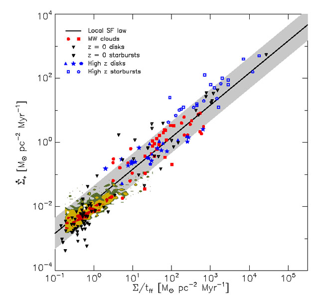Figure 3. SFR per unit area versus gas column density over free-fall time (Krumholz et al. 2012). Different shapes indicate different data sources, and colors represent different types of objects: red circles and squares are Milky Way clouds, black filled triangles and unresolved z = 0 galaxies, black open triangles are unresolved z = 0 starbursts, blue filled symbols are unresolved z > 1 disk galaxies, and blue open symbols are unresolved z > 1 starburst galaxies. Contours show the distribution of kpc-sized regions within nearby galaxies. The black line is ff = 0.01, and the gray band is a factor of 3 range around it.

2.7. GMCs in Varying Galactic Environments

One gains useful insight into GMC physics by studying their properties as a function of environment. Some of the most extreme environments, such as those in starbursts or metal-poor galaxies, also offer unique insights into astrophysics in the primitive universe, and aid in the interpretation of observations of distant sources.

Galactic centers, which feature high metallicity and stellar density, and often high surface densities of gas and star formation, are one unusual environment to which we have observational access. The properties of the bulge, and presence of a bar appear to influence the amount of H₂ in the center (Fisher et al. 2013). Central regions with high _H2 preferentially show reduced _dep(H₂) compared to galaxy averages (Leroy et al. 2013), suggesting that central GMCs convert their gas into stars more rapidly. Reduced _dep(H₂) is correlated with an increase in CO (2-1) / (1-0) ratios, indicating enhanced excitation (or lower optical depth). Many galaxy centers also exhibit a super-exponential increase in CO brightness, and a drop in CO-to-H₂ conversion factor (which reinforces the short _dep(H₂) conclusion, Sandstrom et al. 2012). On the other hand, in our own Galactic Center, Longmore et al. (2013) show that there are massive molecular clouds that have surprisingly little star formation, and depletion times _dep(H₂) ~ 1 Gyr comparable to disk GMCs (Kruijssen et al. 2013), despite volume and column densities orders of magnitude higher (see Longmore et al. Chapter).

Obtaining similar spatially-resolved data on external galaxies is challenging. Rosolowsky and Blitz (2005) examined several very large GMCs (M ~ 10⁷ M, R ~ 40-180 pc) in M 64. They also find a size-linewidth coefficient somewhat larger than in the Milky Way disk, and, in ¹³CO, high surface densities. Recent multi-wavelength, high-resolution ALMA observations of the center of the nearby starburst NGC 253 find cloud masses M ~ 10⁷ M and sizes R ~ 30 pc, implying _GMC 10³ M pc^-2 (Leroy et al. 2013, in prep.). The cloud linewidths imply that they are self-gravitating.

The low metallicity environments of dwarf galaxies and outer galaxy disks supply another fruitful laboratory for study of the influence of environmental conditions. Because of their proximity, the Magellanic Clouds provide the best locations to study metal-poor GMCs. Owing to the scarcity of dust at low metallicity (e.g., Draine et al. 2007) the abundances of H₂ and CO in the ISM are greatly reduced compared to what would be found under comparable conditions in a higher metallicity galaxy (see the discussion in Section 3.3). As a result, CO emission is faint, only being present in regions of very high column density (e.g., Israel et al. 1993, Bolatto et al. 2013 and references therein). Despite these difficulties, there are a number of studies of low metallicity GMCs. Rubio et al. (1993) reported GMCs in the SMC exhibit sizes, masses, and a size-linewidth relation similar to that in the disk of the Milky Way. However, more recent work suggests that GMCs in the Magellanic Clouds are smaller and have lower masses, brightness temperatures, and surface densities than typical inner Milky Way GMCs, although they are otherwise similar to Milky Way clouds (Fukui et al. 2008, Bolatto et al. 2008, Hughes et al. 2010, Muller et al. 2010, Herrera et al. 2013). Magellanic Cloud GMCs also appear to be surrounded by extended envelopes of CO-faint H₂ that are ~ 30% larger than the CO-emitting region (Leroy et al. 2007, Leroy et al. 2009). Despite their CO faintness, though, the SFR-H₂ relation appears to be independent of metallicity once the change in the CO-to-H₂ conversion factor is removed (Bolatto et al. 2011).