7. HIGH-REDSHIFT GALAXIES

The epoch of galaxy formation follows the end of the Dark Ages when baryons could start to accumulate within the DM haloes and star formation was triggered. The scope of this review does not allow us to go into the details of this fascinating subject. Here we shall focus on galaxy evolution during the reionisation epoch, at redshifts z ~ 6-12. We shall not discuss the formation and evolution of the Population III stars either, which has been largely completed by the onset of the reionisation process, except maybe in low-density regions. Section 8 will touch upon some aspects of SMBH formation in 10⁸ M DM haloes. All the problems discussed in the previous sections remain relevant at these high redshifts.

The rapidly increasing list of objects above z ~ 6 makes it possible to study the population of galaxies during reionisation. Deep imaging in multiband surveys using the Wide Field Camera 3 (WFC3) on the HST, as well as some ground-based observations using 8 m telescopes, have revealed galaxies via absorption at wavelengths shorter than Ly from the intervening neutral hydrogen (e.g., Bouwens et al. 2010). In many cases, these photometric redshifts could be verified spectroscopically, up to z ~ 7 (e.g., Pentericci et al. 2011). The majority of reionisation-epoch galaxies are faint, but much rarer brighter galaxies have also been identified at z ~ 8 by means of a large-area medium-deep HST survey (Brightest of Reionizing Galaxies, BoRG) along random lines of sight, including the candidate for the most distant protocluster (Trenti et al. 2011). Even fainter galaxies have been found using gravitational lensing by massive galaxy clusters.

7.1. The high-redshift galaxy zoo

One of the most successful methods to search for reionisation-epoch galaxies is the dropout method based on the absorption short of some characteristic wavelength, the 912 Å Lyman break and a smaller break at Ly 1216 Å, which originate in the intervening neutral hydrogen (e.g., Steidel et al. 1996). Using multiwavelength imaging and filters, objects `disappear' (drop out) when a particular and progressively redder filter is applied. The resulting break in the continuum spectrum allows us to determine the photometric redshift of the object. For z ~ 6, the break lies at ~ 8500 Å. This technique has been applied first to U-band dropouts - galaxies that lack flux in the U-band (z ~ 3), then to g-band dropouts (z ~ 4). The choice of the filter determines the targeted redshift. Additional dropouts have been named according to the relevant bands, i₇₇₅ (z ~ 6), z₈₅₀ (z ~ 7), Y (z ~ 8-9) and J (z ~ 10). Existing data from NICMOS, GOODS/ACS and UDF can reveal dropouts up to z ~ 10. The population of detected galaxies has already provided substantial constraints on the galaxy growth in the Universe at that epoch.

The expanding classification of high-z galaxies has its origin in diverse observational techniques used for their detection and study, resembling the early stages of AGN classification, before unification. Galaxies that exhibit a break in the Lyman continuum redshifted to the UV and other bands have been called Lyman break galaxies (LBGs). Complementary to continuum-selected surveys, the Ly galaxies, or so-called Ly emitters (LAEs), have been mostly detected in narrow-band imaging surveys. Such surveys typically miss the LBGs because of the faint continuum. Spectroscopic identification of z 6 LBGs is only possible if they have strong Ly emission, and are bright (e.g., Vanzella et al. 2011).

An important question is what is the relationship between various classes of high-z galaxy populations and what are their low-z counterparts. Especially interesting is their relationship to sub-mm galaxies, found at z ~ 1-5. These sub-mm galaxies have been detected in the 200 µm - 1 mm band, via redshifted dust emission, using the Sub-mm Common-User Bolometer Array (SCUBA) camera. These objects have a negative K-correction ² because the Rayleigh-Jeans (RJ) tail of the Planck blackbody distribution. Galaxies in the RJ tail become brighter with redshift. They are generally not SBGs because of the weak UV emission. The sub-mm galaxy population consists of very luminous objects with bolometric luminosity ~ 10^12-13 L, emitted mostly in the IR. Powered by intense starbursts, their estimated SFRs are ~ 10^2-3 M yr^-1.

7.2. Mass and luminosity functions

Observations of z 6 galaxies have shown a rapidly evolving galactic LF which agrees with the predicted DM halo mass function (e.g., Bouwens et al. 2011). The UV LF of LBGs has been established with its faint end exhibiting a very steep slope (e.g., Bouwens et al. 2007). Using the Schechter function fit, (L) = (^* / L^*)(L/L^*) exp(-L / L^*), the faint end of this LF at z ~ 7 has the slope of = -1.77 ± 0.20, and ^* = 1.4 × 10^-3 Mpc^-3 mag^-1, which is consistent with no evolution over the time span of z ~ 2-7 (e.g., Oesch et al. 2010). The bright end of the LF evolves significantly over this time period. An even steeper faint end of the LF, = -1.98 ± 0.23, has been claimed recently (Trenti 2012). The SFR appears to decline rapidly with increasing redshift. So by z ~ 6, the number of ionising photons is just enough to keep the Universe ionised, and most of them come from objects fainter than the current detection limit of the HST (e.g., Oesch et al. 2010; Trenti et al. 2010; Trenti 2012).

An accelerated evolution of galaxies during reionisation has been predicted and observed (e.g., Bouwens et al. 2007, 2010; Trenti et al. 2010; Lacey et al. 2011; Oesch et al. 2010, 2012). Strong evolution is expected for z ~ 8-10, by about a factor of ~ 2-5. The estimated number of z ~ 10 galaxies has been derived from the observed LF at z ~ 6 and 8 (Fig. 13). Using this LF, six objects are expected to be present in the field at z ~ 10, but only one has been detected. Hence, the LF appears to drop even faster than expected from the previous empirical lower-redshift extrapolation. The resulting accelerated LF evolution in the range of z ~ 8-10 has been estimated at 94% significance level (Oesch et al. 2012).

Figure 13. UV LFs for z ~ 4, 6, 8 and projected LF at z ~ 10 (Oesch et al. 2012). The z ~ 10 LF extrapolated from fits to lower-redshift LBG LFs is shown as a dashed red line (see also the text). For comparison the z ~ 4 and z ~ 6 LFs are plotted, showing the dramatic buildup of UV luminosity across ~ 1 Gyr of cosmic time. The light-grey vectors along the lower axis indicate the range of luminosities over which the different data sets dominate the z ~ 10 LF constraints.

An important conclusion from the above studies has been the realisation that the UV luminosity density (LD) originating in the high-z galaxy population levels off and gradually falls toward higher z, in the range z ~ 3-8 (Fig. 14). The LD data at z ~ 4-8 are taken from Bouwens et al. (2007) and Bouwens et al. (2011). As can be seen in Fig. 14, the LD increases by more than an order of magnitude in 170 Myr from z ~ 10 to 8, indicating that the galaxy population at this luminosity range evolves by a factor 4 more than expected from low-redshift extrapolations. The predicted LD evolution of the semi-analytical model of Lacey et al. (2011) is shown as a dashed blue line, and the prediction from theoretical modelling (Trenti et al. 2010) is shown as a blue solid line. These reproduce the expected LD at z ~ 10 remarkably well.

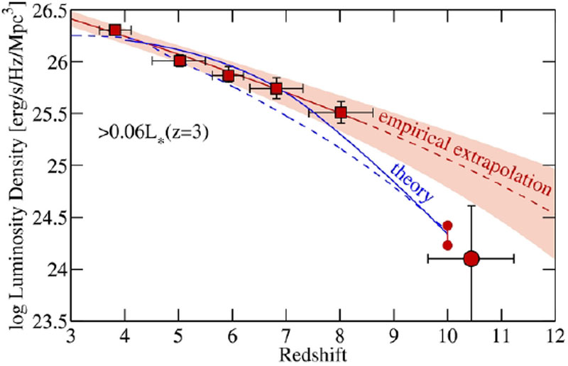Figure 14. Evolution of the UV LD above M1400 = -18 mag [> 0.06 L*(z = 3)] (Oesch et al. 2012). The filled circle at z ~ 10.4 is the LD directly measured for the galaxy candidate. The red line corresponds to the empirical LF evolution. Its extrapolation to z > 8 is shown as a dashed red line.

Analysis and modelling of the available data point to the underlying cause: the accelerated evolution is driven by changes in the DM halo mass function (HMF), as follows from theoretical considerations (e.g., Trenti et al. 2010) and semi-analytical modelling (e.g., Lacey et al. 2011), and not by the star formation processes in these galaxies. Interestingly, the rapid assembly of haloes at z ~ 8-10 alone can explain the LF evolution (Trenti et al. 2010). However, this assumption has never been put to a self-consistent test using high-resolution simulations with the relevant baryon physics. The possible link between LF and the DM HMF has been studied by means of the conditional LF method (e.g., Trenti et al. 2010 and references therein) to understand the processes regulating star formation. The main conclusions can be summarised as (1) a significant redshift evolution of galaxy luminosity vs halo mass, L_gal(M_h), (2) only a fraction ~ 20-30% appear to host LBGs, and (3) the LF for z 6 deviates from the Schechter functional form, in particular, by missing the sharp drop in density of luminous M -20 galaxies with L. For example, due to the short timescales - z ~ 1 corresponds to 170 Mpc - it becomes difficult to rely on the fast evolution of L_gal(M_h), while M_h evolves rapidly at these redshifts.

Due to the nature of the hierarchical growth of structure, high-z galaxies should appear and grow fastest in the highest overdensities, and therefore are expected to be strongly clustered around the density peaks. For example, Trenti et al. (2012) infer the properties of DM haloes in the BoRG 58 field at z ~ 8 based on the found five Y₀₉₈-dropouts, using the Improved Conditional Luminosity Function model. The brightest member of the associated overdensity appears to reside in a halo of ~ (4-7 ± 2) × 10¹¹ M - a 5 density peak which corresponds to a comoving space density of ~ (9-15) × 10^-7 Mpc^-3. It has ~ 20-70% chance of being present within the volume probed by the BoRG survey. Using an extended Press-Schechter function, about 4.8 haloes more massive than 10¹¹ M are expected in the associated region with the (comoving) radius of 1.55 Mpc, compared to less than 10^-3 in the random region. For higher accuracy, a set of 10 cosmological simulations (Romano-Díaz et al. 2011a) has been used, tailored to study high-z galaxy formation in such an over-dense environment. A DM mass resolution of 3 × 10⁸ M has been used, and, therefore, haloes with masses 10¹¹ M have been well resolved. The constrained realisation (CR) method (e.g., Bertschinger 1987; Hoffman & Ribak 1991; Romano-Díaz et al. 2007, 2009, 2011a, b) has been instrumental in modelling these rare over-dense regions. We describe this method below.

The CR method consists of a series of linear constraints on the initial density field used to design prescribed initial conditions. It is not an approximation but an exact method. All the constraints are of the same form - the value of the initial density field at different locations, and are evaluated with different Gaussian smoothing kernels, with their width fixed so as to encompass the mass scale on which a constraint is imposed. The set of mass scales and the location at which the constraints are imposed define the numerical experiment. Assuming a cosmological model and power spectrum of the primordial perturbation field, a random realisation of the field is constructed from which a CR is generated. The additional use of the zoom-in technique assures that the high-resolution region of simulations is subject to large-scale gravitational torques. The CRs provide a unique tool to study high-z galaxies at an unprecedented resolution. It allows one to use much smaller cosmological volumes, and, without any loss of generality, accounts for the cosmic variance.

The initial conditions for the test runs described above have been constrained to have a halo of mass ~ 10¹² M by z ~ 6. This halo has reached ~ 5 × 10¹¹ M by z ~ 8 in compliance with BoRG 58-17871420. Within the field of view of 70" × 70" and the redshift depth of z ~ 19 Mpc about 6.4 haloes more massive than ~ 10¹¹ M have been expected, and the highest number found in the simulations was 10 (Fig. 15). A random (unconstrained) region of the same volume has been estimated to host ~ 0.013 such haloes. The probability of contamination in such a small area is negligible, ~ 2.5 × 10^-4. In summary, if indeed the brightest member of the BoRG 58 field lives in a massive DM halo, the fainter dropouts detected in this field are part of the overdensity that contributes to the protocluster, depending of course on spectroscopic confirmation. Simulations provide some insight into the fate of this overdensity with a total DM mass of ~ (1-2) × 10¹³ M - it has collapsed by z ~ 3, and is expected to grow to ~ (1-2) × 10¹⁴ M by z = 0.

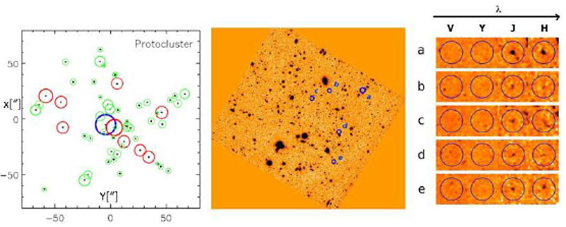Figure 15. The most distant candidate protocluster at z ~ 8 (Trenti et al. 2012). Left: DM halo distribution for a simulated protocluster in a comoving volume of 11 × 11 × 19 Mpc3 from Romano-Díaz et al. (2011a). The largest (blue) circle represents the most massive halo in the simulation, ~ 5 × 1011 M; red circles, haloes above 1011 M; green circles, haloes of 1010-1011 M. Middle: J125 image of BoRG 58 field, with Y098-dropouts indicated by (blue) circles. Right: Postage-stamp images (3.2" × 3.2") of sources: BoRG 58-17871420, BoRG 58-14061418, BoRG 58-12071332, BoRG 58-15140953, and BoRG 58-14550613 fields (top to bottom).

The evolution of the HMF is very sensitive to the assumed cosmology, because the halo growth rate depends on the average matter density in the Universe. As the DM is not observable directly, numerical simulations are indispensable in studying the halo growth, and analytic techniques provide an additional tool. The process of DM halo formation quickly becomes non-linear which makes an analytical follow-up difficult. Analytically, one relies on modelling the spherical or ellipsoidal collapses, but only N-body simulations reveal the complexity of the process which is hierarchical in Nature. Numerically, the halo growth depends on the force resolution used and on the size of the computational box. The N-body simulations of halo evolution are very accurate, ~ 1%, and the analytical methods are ~ 10-20% (e.g., Press & Schechter 1974, Bond et al. 1991). Nevertheless, the analytical HMF can reproduce the numerical results at least qualitatively, and can be defined ³ as dn / dM, where n(M) is the number density of haloes in the range dM around mass M at redshift z (e.g., Jenkins et al. 2001),

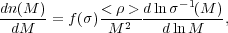(10)

where ² is the variance of the (linear) density field smoothed on the scale corresponding to M, and <> is the average density in the Universe. In the spherical collapse approximation developed by Press & Schechter (1974), f() = (2 / )^1/2(_c / ) exp(-_c² / 2²), where _c 1.686. Press & Schechter assumed that all the mass is within the DM haloes, i.e., ∫_-∞^+∞ f()d ln ^-1 = 1. An extension for arbitrary redshift is achieved by taking _c = _c(z = 0) / D(z), D(z) being the linear growth factor.

Discrepancies between the analytically derived and numerically obtained HMFs can be sufficient to affect our understanding of galaxy growth during the reionisation epoch, as shown in Fig. 16 (Lukic et al. 2007). It is, therefore, important that the shape of the HMF can have a universal character, independent of epoch, cosmological parameters and the initial power spectrum, in particular representations (Jenkins et al. 2001), although this must be taken with caution. Violations of universality have been found both at low (z 5 at ~ 20% level, Fig. 16), and high (z ~ 10-30) redshifts, but the issue is still unsettled due a number of numerical concerns (e.g., Lukic et al. 2007; Reed et al. 2007).

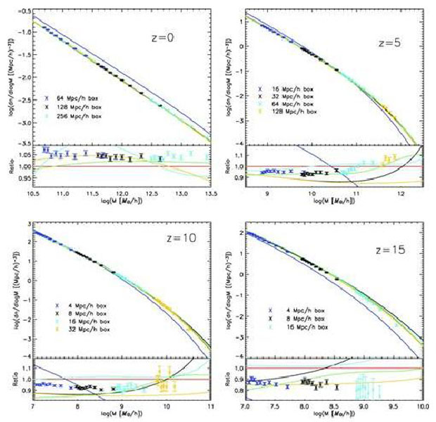Figure 16. The HMFs at four redshifts (z = 0, 5, 10 and 15) compared to different fitting formulae, analytic and numerical (coloured curves). Note that the mass ranges are different at different redshifts. The bottom panels show the ratio with respect to the Warren et al. (2006) fit, agreeing at the 10% level for z 10, and with a systematic offset of 5% at z = 0. At higher redshifts, agreement is at the 20% level. Agreement becomes very close once finite-volume corrections are applied. Press-Schechter is a bad fit at all redshifts, especially at high redshifts, z 10, where the difference is an order of magnitude. From Lukic et al. (2007).

² The K-correction is the dimming of a source due to the 1 + z shift of the wavelength band and its width. Back.

³ A variety of definitions of the HMF exist in the literature. We use the differential HMF. Back.