2. BAYESIAN PROBABILITY THEORY

In this section we introduce the basic concepts and the notation we employ. After a discussion of what probability is, we turn to the central formula for Bayesian inference, namely Bayes theorem. The whole of Bayesian inference follows from this extremely simple cornerstone. We then present some views about the meaning of priors and their role in Bayesian theory, an issue which has always been (wrongly) considered a weak point of Bayesian statistics.

There are many excellent textbooks on Bayesian statistics: the works by Sir Harold Jeffreys [3] and Bruno de Finetti [4] are classics, while an excellent modern introduction with an extensive reading list is given by [5]. A good textbook is [6]. Worth reading as a source of inspiration is the though-provoking monograph by E.T. Jaynes [7]. Computational aspects are treated in [8], while MacKay [9] has a quite unconventional but inspiring choice of topics with many useful exercices. Two very good textbooks on the subject written by physicists are [10, 11]. A nice introductory review aimed at physicists is [12] (see also [13]). Tom Loredo has some masterfully written introductory material, too [14, 15]. A good source expanding on many of the topics covered here is Ref. [16].

2.1. What is probability?

2.1.1. Probability as frequency. The classical approach to statistics defines the probability of an event as

"the number of times the event occurs over the total number of trials, in the limit of an infinite series of equiprobable repetitions."

This is the so-called frequentist school of thought. This definition of probability is however unsatisfactory in many respects.

1. Strikingly, this definition of probability in terms of relative frequency of outcomes is circular, i.e. it assumes that repeated trials have the same probability of outcomes - but it was the the very notion of probability that we were trying to define in the first place!
2. It cannot handle with unrepeatable situations, such as the probability that I will be overrun by a car when crossing the street, or, in the cosmological context, questions concerning the properties of the observable Universe as a whole, of which we have exactly one sample. Indeed, perfectly legitimate questions such as "what is the probability that it was raining in Oxford when William I was crowned?" cannot even be formulated in classical statistics.
3. The definition only holds exactly for an infinite sequence of repetitions. In practice we always handle with a finite number of measurements, sometimes with actually only a very small number of them. How can we assess when "how many repetitions" are sufficient? And what shall we do when we have only a handful of repetitions? Frequentist statistics does not say, except sometimes devising complicated ad-hockeries to correct for "small sample size" effects. In practice, physicists tend to forget about the "infinite series" requirement and use this definitions and the results that go with it (for example, about asymptotic distributions of test statistics) for whatever number of samples they happen to be working with.

Another, more subtle aspects has to do with the notion of "randomness". Restricting ourselves to classical (non-chaotic) physical systems for now, let us consider the paradigmatic example of a series of coin tosses. From an observed sequence of heads and tails we would like to come up with a statistical statement about the fairness of the coin, which is deemed to be "fair" if the probability of getting heads is p_H = 0.5. At first sight, it might appear plausible that the task is to determine whether the coin possesses some physical property (for example, a tensor of intertia symmetric about the plane of the coin) that will ensure that the outcome is indifferent with respect to the interchange of heads and tails. As forcefully argued by Jaynes [7], however, the probability of the outcome of a sequence of tosses has nothing to do with the physical properties of the coin being tested! In fact, a skilled coin-tosser (or a purpose-built machine, see [17]) can influence the outcome quite independently of whether the coin is well-balanced (i.e., symmetric) or heavily loaded. The key to the outcome is in fact the definition of random toss. In a loose, intuitive fashion, we sense that a carefully controlled toss, say in which we are able to set quite precisely the spin and speed of the coin, will spoil the "randomness" of the experiment — in fact, we might well call it "cheating". However, lacking a precise operational definition of what a "random toss" means, we cannot meaningfully talk of the probability of getting heads as of a physical property of the coin itself. It appears that the outcome depends on our state of knowledge about the initial conditions of the system (angular momentum and velocity of the toss): an lack of precise information about the initial conditions results in a state of knowledge of indifference about the possible outcome with respect to the specification of heads or tails. If however we insist on defining probability in terms of the outcome of random experiments, we immediately get locked up in a circularity when we try to specify what "random" means. For example, one could say that

"a random toss is one for which the sequence of heads and tails is compatible with assuming the hypothesis p_H = 0.5".

But the latter statement is exactly what we were trying to test in the first place by using a sequence of random tosses! We are back to the problem of circular definition we highlighted above.

2.1.2. Probability as degree of belief. Many of the limitations above can be avoided and paradoxes resolved by taking a Bayesian stance about probabilities. The Bayesian viewpoint is based on the simple and intuitive tenet that

"probability is a measure of the degree of belief about a proposition".

It is immediately clear that this definition of probability applies to any event, regardless whether we are considering repeated experiments (e.g., what is the probability of obtaining 10 heads in as many tosses of a coin?) or one-off situations (e.g., what is the probability that it will rain tomorrow?). Another advantage is that it deals with uncertainty independently of its origin, i.e. there is no distinction between "statistical uncertainty" coming from the finite precision of the measurement apparatus and the associated random noise and "systematic uncertainty", deriving from deterministic effects that are only partially known (e.g., calibration uncertainty of a detector). From the coin tossing example above we learn that it makes good sense to think of probability as a state of knowledge in presence of partial information and that "randomness" is really a consequence of our lack of information about the exact conditions of the system (if we knew the precise way the coin is flipped we could predict the outcome of any toss with certainty. The case of quantum probabilities is discussed below). The rule for manipulating states of belief is given by Bayes' Theorem, which is introduced in Eq. (5) below.

It seems to us that the above arguments strongly favour the Bayesian view of probability (a more detailed discussion can be found in [7, 14]). Ultimately, as physicists we might as well take the pragmatic view that the approach that yields demonstrably superior results ought to be preferred. In many real-life cases, there are several good reasons to prefer a Bayesian viewpoint:

1. Classic frequentist methods are often based on asymptotic properties of estimators. Only a handful of cases exist that are simple enough to be amenable to analytic treatment (in physical problems one most often encounters the Normal and the Poisson distribution). Often, methods based on such distributions are employed not because they accurately describe the problem at hand, but because of the lack of better tools. This can lead to serious mistakes. Bayesian inference is not concerned by such problems: it can be shown that application of Bayes' Theorem recovers frequentist results (in the long run) for cases simple enough where such results exist, while remaining applicable to questions that cannot even be asked in a frequentist context.
2. Bayesian inference deals effortlessly with nuisance parameters. Those are parameters that have an influence on the data but are of no interest for us. For example, a problem commonly encountered in astrophysics is the estimation of a signal in the presence of a background rate (see [14, 18, 19]). The particles of interest might be photons, neutrinos or cosmic rays. Measurements of the source s must account for uncertainty in the background, described by a nuisance parameter b. The Bayesian procedure is straightforward: infer the joint probability of s and b and then integrate over the uninteresting nuisance parameter b ("marginalization", see Eq. (16)). Frequentist methods offer no simple way of dealing with nuisance parameters (the very name derives from the difficulty of accounting for them in classical statistics). However neglecting nuisance parameters or fixing them to their best-fit value can result in a very serious underestimation of the uncertainty on the parameters of interest (see [20] for an example involving galaxy evolution models).
3. In many situations prior information is highly relevant and omitting it would result in seriously wrong inferences. The simplest case is when the parameters of interest have a physical meaning that restricts their possible values: masses, count rates, power and light intensity are examples of quantities that must be positive. Frequentist procedures based only on the likelihood can give best-fit estimates that are negative, and hence meaningless, unless special care is taken (for example, constrained likelihood methods). This often happens in the regime of small counts or low signal to noise. The use of Bayes' Theorem ensures that relevant prior information is accounted for in the final inference and that physically meaningless results are weeded out from the beginning.
4. Bayesian statistics only deals with the data that were actually observed, while frequentist methods focus on the distribution of possible data that have not been obtained. As a consequence, frequentist results can depend on what the experimenter thinks about the probability of data that have not been observed. (this is called the "stopping rule" problem). This state of affairs is obviously absurd. Our inferences should not depend on the probability of what could have happened but should be conditional on whatever has actually occurred. This is built into Bayesian methods from the beginning since inferences are by construction conditional on the observed data.

However one looks at the question, it is fair to say that the debate among statisticians is far from settled (for a discussion geared for physicists, see [21]). Louis Lyons neatly summarized the state of affairs by saying that [22]

"Bayesians address the question everyone is interested in by using assumptions no-one believes, while frequentists use impeccable logic to deal with an issue of no interest to anyone".

2.1.3. Quantum probability. Ultimately the quantum nature of the microscopic world ensures that the fundamental meaning of probability is to be found in a theory of quantum measurement. The fundamental problem is how to make sense of the indeterminism brought about when the wavefunction collapses into one or other of the eigenstates being measured. The classic textbook view is that the probability of each outcome is given by the square of the amplitude, the so-called "Born rule". However the question remains — where do quantum probabilities come from?

Recent developments have scrutinized the scenario of the Everettian many-worlds interpretation of quantum mechanics, in which the collapse never happens but rather the world "splits" in disconnected "branches" every time a quantum measurement is performed. Although all outcomes actually occur, uncertainty comes into the picture because an observer is unsure about which outcome will occur in her branch. David Deutsch [23] suggested to consider the problem from a decision-theoretic point of view. He proposed to consider a formal system in which the probabilities ("weights") to be assigned to each quantum branch are expressed in terms of the preferences of a rational agent playing a quantum game. Each outcome of the game (i.e., weights assignment) has an associated utility function that determines the payoff of the rational agent. Being rational, the agent will act to maximise the expectation value of her utility. The claim is that it is possible to find a simple and plausible set or rules for the quantum game that allow to derive unique outcomes (i.e., probability assignments) in agreement with the Born rule, independently of the utility function chosen, i.e. the payoffs. In such a way, one obtains a bridge between subjective probabilities (the weight assignment by the rational agent) and quantum chance (the weights attached to the branches according to the Born rule).

This approach to the problem of quantum measurement remains highly controversial. For an introduction and further reading, see e.g. [24, 25] and references therein. An interesting comparison between classical and quantum probabilities can be found in [26].

2.2. Bayes' Theorem

Bayes' Theorem is a simple consequence of the axioms of probability theory, giving the rules by which probabilities (understood as degree of belief in propositions) should be manipulated. As a mathematical statement it is not controversial — what is a matter of debate is whether it should be used as a basis for inference and in general for dealing with uncertainty. In the previous section we have given some arguments why we strongly believe this to be the case. An important result is that Bayes' Theorem can be derived from a set of basic consistency requirements for plausible reasoning, known as Cox axioms [27]. Therefore, Bayesian probability theory can be shown to be the unique generalization of boolean logic into a formal system to manipulate propositions in the presence of uncertainty [7]. In other words, Bayesian inference is the unique generalization of logical deduction when the available information is incomplete.

We now turn to the presentation of the actual mathematical framework. We adopt a fairly relaxed notation, as mathematical rigour is not the aim of this review. For a more formal introduction, see e.g. [3, 7].

Let us consider a proposition A, which could be a random variable (e.g., the probability of obtaining 12 when rolling two dices) or a one-off proposition (the probability that Prince Charles will become king in 2015), and its negation, A. The sum rule reads

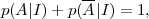(1)

where the vertical bar means that the probability assignment is conditional on assuming whatever information is given on its right. Above, I represents any relevant information that is assumed to be true. The product rule is written as

(2)

which says that the joint probability of A and B equals to the probability of A given that B occurs times the probability of B occurring on its own (both conditional on information I). If we are interested in the probability of B alone, irrespective of A, the sum and product rules together imply that

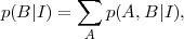(3)

where the sum runs over the possible outcomes for proposition A. The quantity on the left-hand-side is called marginal probability of B. Since obviously p(A,B|I) = p(B,A|I), the product rule can be rewritten to give Bayes' Theorem:

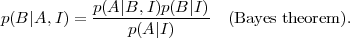(4)

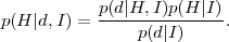
The interpretation of this simple result is more illuminating if one replaces for A the observed data d and for B the hypothesis H we want to assess, obtaining

(5)

On the left-hand side, p(H | d, I) is the posterior probability of the hypothesis taking the data into account. This is proportional to the sampling distribution of the data p(d | H,I) assuming the hypothesis is true, times the prior probability for the hypothesis, p(H | I) ("the prior", conditional on whatever external information we have, I), which represents our state of knowledge before seeing the data. The sampling distribution encodes how the degree of plausibility of the hypothesis changes when we acquire new data. Considered as a function of the hypothesis, for fixed data (the ones that have been observed), it is called the likelihood function and we will often employ the shortcut notation (H) p(d | H,I). Notice that as a function of the hypothesis the likelihood is not a probability distribution. The normalization constant on the right-hand-side in the denominator is the marginal likelihood (in cosmology often called the "Bayesian evidence") given by

(6)

where the sum runs over all the possible outcomes for the hypothesis H. This is the central quantity for model comparison purposes, and it is further discussed in section 4. The posterior is the relevant quantity for Bayesian inference as it represents our state of belief about the hypothesis after we have considered the information in the data (hence the name). Notice that there is a logical sequence in going from the prior to the posterior, not necessarily a temporal one, i.e. a scientist might well specify the prior after the data have been gathered provided that the prior reflects her state of knowledge irrespective of the data. Bayes' Theorem is therefore a prescription as to how one learns from experience. It gives a unique rule to update one's beliefs in the light of the observed data.

The need to specify a prior describing a "subjective" state of knowledge has exposed Bayesian inference to the criticism that it is not objective, and hence unfit for scientific reasoning. Exactly the contrary is true — a thorny issue to which we now briefly turn out attention.

2.3. Subjectivity, priors and all that

The prior choice is a fundamental ingredient of Bayesian statistics. Historically, it has been regarded as problematic, since the theory does not give guidance about how the prior should be selected. Here we argue that this issue has been given undue emphasis and that prior specification should be regarded as a feature of Bayesian statistics, rather than a limitation.

The guiding principle of Bayesian probability theory is that there can be no inference without assumptions, and thus the prior choice ought to reflect as accurately as possible one's assumptions and state of knowledge about the problem in question before the data come along. Far from undermining objectivity, this is obviously a positive feature, because Bayes' Theorem gives a univoque procedure to update different degrees of beliefs that different scientist might have held before seeing the data. Furthermore, there are many cases where prior (i.e., external) information is relevant and it is sensible to include it in the inference procedure ¹.

It is only natural that two scientists might have different priors as a consequence of their past scientific experiences, theoretical outlook and based on the outcome of previous observations they might have performed. As long as the prior p(H|I) (where the extra conditioning on I denotes the external information of the kind listed above) has a support that is non-zero in regions where the likelihood is large, repeated application of Bayes theorem, Eq. (5), will lead to a posterior pdf that converges to a common, i.e. objective inference on the hypothesis. As an example, consider the case where the inference concerns the value of some physical quantity , in which case p( | d, I) has to be interpreted as the posterior probability density and p( | d, I) d is the probability of to take on a value between and + d . Alice and Bob have different prior beliefs regarding the possible value of , perhaps based on previous, independent measurements of that quantity that they have performed. Let us denote their priors by p( | I_i) (i = A,B) and let us assume that they are described by two Gaussian distributions of mean µ_i and variance _i², i = A,B representing the state of knowledge of Alice and Bob, respectively. Alice and Bob go together in the lab and perform a measurement of with an apparatus subject to Gaussian noise of known variance ². They obtain a value m₁, hence their likelihood is

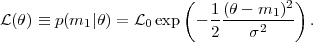(7)

Replacing the hypothesis H by the continuous variable in Bayes' Theorem ², we obtain for their respective posterior pdf's after the new datum

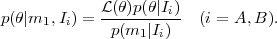(8)

It is easy to see that the posterior pdf's of Alice and Bob are again Gaussians with means

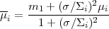(9)

and variance

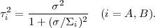(10)

Thus if the likelihood is more informative than the prior, i.e. for ( / _i) ≪ 1 the posterior means of Bob and Alice will converge towards the measured value, m₁. As more and more data points are gathered, one can simply replace m₁ in the above equations by the mean m of the observations and ² by ² / N, with N the number of data points. Thus we can see that the initial prior means µ_i of Alice and Bob will progressively be overridden by the data. This process is illustrated in Figure 2.

Figure 2. Converging views in Bayesian inference. Two scientists having different prior believes p( | Ii) about the value of a quantity (panel (a), red and green pdf's) observe one datum with likelihood () (panel (b)), after which their posteriors p( | m1) (panel (c), obtained via Bayes Theorem, Eq. (8)) represent their updated states of knowledge on the parameter. After observing 100 data points, the two posteriors have become essentially indistinguishable (d).

The situation is somewhat different for model comparison questions. In this case, it is precisely the available prior volume that is important in determining the penalty that more complex models with more free parameters should incur into (this is discussed in detail in section 4). Hence the impact of the prior choice is much stronger when dealing with model selection issues, and care should be exercised in assessing how much the outcome would change for physically reasonable changes in the prior.

There is a vast literature on priors that we cannot begin to summarize here. Important issues concern the determination of "ignorance priors", i.e. priors reflecting a state of indifference with respect to symmetries of the problem considered. "Reference priors" exploit the idea of using characteristics of what the experiment is expected to provide to construct priors representing the least informative state of knowledge. In order to be probability distributions, priors must be proper, i.e. normalizable to unity probability content. "Flat priors" are often a standard choice, in which the prior is taken to be constant within some minimum and maximum value of the parameters, i.e. for a 1-dimensional case p() = (_max - _min)^-1. The rationale is that we should assign equal probability to equal states of knowledge. However, flat priors are not always as harmless as they appear. One reason is that a flat prior on a parameter does not correspond to a flat prior on a non-linear function of that parameter, (). The two priors are related by

(11)

so for a non-linear dependence () the term |d / d | means that an uninformative (flat) prior on might be strongly informative about (in the multi-dimensional case, the derivative term is replaced by the determinant of the Jacobian for the transformation). Furthermore, if we are ignorant about the scale of a quantity , it can be shown (see e.g. [7]) that the appropriate prior is flat on ln, which gives equal weight to all orders of magnitude. This prior corresponds to p() ∝ ^-1 and is called "Jeffreys' prior". It is appropriate for example for the rate of a Poisson distribution. For further details on prior choice, and especially so-called "objective priors", see e.g. chapter 5 in [28] and references therein.

¹ As argued above, often it would be a mistake not to do so, for example when trying to estimate a mass m from some data one should enforce it to be a positive quantity by requiring that p(m) = 0 for m < 0. Back.

² Strictly speaking, Bayes' Theorem holds for discrete probabilities and the passage to hypotheses represented by continuous variables ought to be performed with some mathematical care. Here we simply appeal to the intuition of physicists without being too much concerned by mathematical rigour. Back.