


4.1. Shaving theories with Occam's razor
When there are several competing theoretical models, Bayesian model comparison provides a formal way of evaluating their relative probabilities in light of the data and any prior information available. The "best" model is then the one which strikes an optimum balance between quality of fit and predictivity. In fact, it is obvious that a model with more free parameters will always fit the data better (or at least as good as) a model with less parameters. However, more free parameters also mean a more "complex" model, in a sense that we will quantify below in section 4.6. Such an added complexity ought to be avoided whenever a simpler model provides an adequate description of the observations. This guiding principle of simplicity and economy of an explanation is known as Occam's razor — the simplest theory compatible with the available evidence ought to be preferred 3. Bayesian model comparison offers a formal way to evaluate whether the extra complexity of a model is required by the data, thus putting on a firmer statistical grounds the evaluation and selection process of scientific theories that scientists often carry out at a more intuitive level. For example, a Bayesian model comparison of the Ptolemaic model of epicycles versus the heliocentric model based on Newtonian gravity would favour the latter because of its simplicity and ability to explain planetary motions in a more economic fashion than the baroque construction of epicycles.
An important feature is that an alternative model must be specified against which the comparison is made. In contrast with frequentist goodness-of-fit tests (such as chi-square tests), Bayesian model comparison maintains that it is pointless to reject a theory unless an alternative explanation is available that fits the observed facts better (for more details about the difference in approach with frequentist hypothesis testing, see [14]). In other words, unless the observations are totally impossible within a model, finding that the data are improbable given a theory does not say anything about the probability of the theory itself unless we can compare it with an alternative. A consequence of this is that the probability of a theory that makes a correct prediction can increase if the prediction is confirmed by observations, provided competitor theories do not make the same prediction. This agrees with our intuition that a verified prediction lends support to the theory that made it, in contrast with the limited concept of falsifiability advocated by Popper (i.e., that scientific theories can only be tested by proving them wrong). So for example, perturbations to the motion of Uranus led the French astronomer U.J.J Leverrier and the English scholar J.C. Adams to formulate the prediction, based on Newtonian theory, that a further planet ought to exist beyond the orbit of Uranus. The discovery of Neptune in 1846 within 1 degree of the predicted position thus should strengthen our belief in the correctness of Newtonian gravity. However, as discussed in detail in chapter 5 of Ref [7], the change in the plausibility of Newton's theory following the discovery of Uranus crucially depends on the alternative we are considering. If the alternative theory is Einstein gravity, then obviously the two theories make the same predictions as far as the orbit of Uranus is concerned, hence their relative plausibility is unchanged by the discovery. The alternative "Newton theory is false" is not useful in Bayesian model comparison, and we are forced to put on the table a more specific model than that before we can assess how much the new observation changes our relative degree of belief between an alternative theory and Newtonian gravity.
In the context of model comparison it is appropriate to think of a
model as a specification of a set of parameters
 and of
their prior distribution,
p( |
and of
their prior distribution,
p( |
 ). As shown
below, it is the number of free parameters and their prior
range that control the strength of the Occam's razor effect in
Bayesian model comparison: models that have many parameters that
can take on a wide range of values but that are not needed in the
light of the data are penalized for their unwarranted complexity.
Therefore, the prior choice ought to reflect the available
parameter space under the model
, independently of
experimental constraints we might already be aware of. This is
because we are trying to assess the economy (or simplicity) of the
model itself, and hence the prior should be based on theoretical
or physical constraints on the model under consideration. Often
these will take the form of a range of values that are deemed
"intuitively" plausible, or "natural". Thus the prior
specification is inherent in the model comparison approach.
). As shown
below, it is the number of free parameters and their prior
range that control the strength of the Occam's razor effect in
Bayesian model comparison: models that have many parameters that
can take on a wide range of values but that are not needed in the
light of the data are penalized for their unwarranted complexity.
Therefore, the prior choice ought to reflect the available
parameter space under the model
, independently of
experimental constraints we might already be aware of. This is
because we are trying to assess the economy (or simplicity) of the
model itself, and hence the prior should be based on theoretical
or physical constraints on the model under consideration. Often
these will take the form of a range of values that are deemed
"intuitively" plausible, or "natural". Thus the prior
specification is inherent in the model comparison approach.
The prime tool for model selection is the Bayesian evidence, discussed in the next three sections. A quantitative measure of the effective model complexity is introduced in section 4.6. We then present some popular approximations to the full Bayesian evidence that attempt to avoid the difficulty of priors choice, the information criteria, and discuss the limits of their applicability in section 4.7.
For reviews on model selection see e.g. [3, 38, 9] and [39] for cosmological applications. Good starting points on Bayes factors are [40, 41]. A discussion of the spirit of model selection can be found in the first part of [42].
The evaluation of a model's performance in the light of the data
is based on the Bayesian evidence, which in the statistical
literature is often called marginal likelihood or model
likelihood. Here we follow the practice of the cosmology and
astrophysics community and will use the term "evidence" instead.
The evidence is the normalization integral on the
right-hand-side of Bayes' theorem, Eq. (6),
which we rewrite here for a continuous parameter space
 and
conditioning explicitly on the model under
consideration, :
and
conditioning explicitly on the model under
consideration, :
 |
(17) |
Thus the Bayesian evidence is the average of the likelihood under the prior for a specific model choice. From the evidence, the model posterior probability given the data is obtained by using Bayes' Theorem to invert the order of conditioning:
 |
(18) |
where we have dropped an irrelevant normalization constant that
depends only on the data and
p() is the prior
probability assigned to the model itself. Usually this is taken to be
non-committal and equal to 1 / Nm if one considers
Nm different models. When comparing two models,
0 versus
1, one is
interested in the ratio of the posterior
probabilities, or posterior odds, given by
 |
(19) |
and the Bayes factor B01 is the ratio of the models' evidences:
 |
(20) |
A value B01 > (<) 1 represents an increase (decrease) of the support in favour of model 0 versus model 1 given the observed data. From Eq. (19) it follows that the Bayes factor gives the factor by which the relative odds between the two models have changed after the arrival of the data, regardless of what we thought of the relative plausibility of the models before the data, given by the ratio of the prior models' probabilities. Therefore the relevant quantity to update our state of belief in two competing models is the Bayes factor.
To gain some intuition about how the Bayes factor works, consider
two competing models:
0 predicting
that a quantity = 0
with no free parameters, and
1 which assigns
a Gaussian prior distribution with 0 mean and variance
 2.
Assume we perform a measurement of
described by a normal
likelihood of standard deviation
2.
Assume we perform a measurement of
described by a normal
likelihood of standard deviation
 , and with the maximum
likelihood value lying
, and with the maximum
likelihood value lying  standard deviations away from 0,
i.e. |max /
| =
. Then the Bayes factor
between the two models is given by, from Eq. (20)
standard deviations away from 0,
i.e. |max /
| =
. Then the Bayes factor
between the two models is given by, from Eq. (20)
 |
(21) |
For
≫ 1, corresponding to a detection of the new
parameter at many sigma, the exponential term dominates and
B01 ≪ 1, favouring the more complex model with a
non-zero
extra parameter, in agreement with the usual conclusion. But if
 1 and
/
≪ 1
(i.e., the likelihood
is much more sharply peaked than the prior and in the vicinity of
0), then the prediction of the simpler model that
= 0 has
been confirmed. This leads to the Bayes factor being dominated by
the Occam's razor term, and B01
≈ /
, i.e.
evidence accumulates in favour of the simpler model proportionally
to the volume of "wasted" parameter space. If however
/
≫ 1
then the likelihood is less informative than
the prior and B01 → 1, i.e. the data have not
changed our relative belief in the two models.
1 and
/
≪ 1
(i.e., the likelihood
is much more sharply peaked than the prior and in the vicinity of
0), then the prediction of the simpler model that
= 0 has
been confirmed. This leads to the Bayes factor being dominated by
the Occam's razor term, and B01
≈ /
, i.e.
evidence accumulates in favour of the simpler model proportionally
to the volume of "wasted" parameter space. If however
/
≫ 1
then the likelihood is less informative than
the prior and B01 → 1, i.e. the data have not
changed our relative belief in the two models.
Bayes factors are usually interpreted against the Jeffreys' scale [3] for the strength of evidence, given in Table 1. This is an empirically calibrated scale, with thresholds at values of the odds of about 3:1, 12:1 and 150:1, representing weak, moderate and strong evidence, respectively. A useful way of thinking of the Jeffreys' scale is in terms of betting odds — many of us would feel that odds of 150:1 are a fairly strong disincentive towards betting a large sum of money on the outcome. Also notice from Table 1 that the relevant quantity in the scale is the logarithm of the Bayes factor, which tells us that evidence only accumulates slowly and that indeed moving up a level in the evidence strength scale requires about an order of magnitude more support than the level before.
| |ln B01| | Odds | Probability | Strength of evidence |
| <1.0 |
3:1 |
<0.750 | Inconclusive |
| 1.0 | ~ 3:1 | 0.750 | Weak evidence |
| 2.5 | ~ 12:1 | 0.923 | Moderate evidence |
| 5.0 | ~ 150:1 | 0.993 | Strong evidence |
Bayesian model comparison does not replace the parameter inference step (which is performed within each of the models separately). Instead, model comparison extends the assessment of hypotheses in the light of the available data to the space of theoretical models, as evident from Eq. (19), which is the equivalent expression for models to Eq. (12), representing inference about the parameters value within each model (for multi-model inference, merging the two levels, see section 6.2).
4.3. Computation and interpretation of the evidence
The computation of the Bayesian evidence (17) is in general a numerically challenging task, as it involves a multi-dimensional integration over the whole of parameter space. An added difficulty is that the likelihood is often sharply peaked within the prior range, but possibly with long tails that do contribute significantly to the integral and which cannot be neglected. Other problematic situations arise when the likelihood is multi-modal, or when it has strong degeneracies that confine the posterior to thin sheets in parameter space. Until recently, the application of Bayesian model comparison has been hampered by the difficulty of reliably estimating the evidence. Fortunately, several methods are now available, each with its own strengths and domains of applicability.
1) reduces to
the original model
(0) for specific
values of the new parameters. This is a fairly common scenario in
cosmology, where one wishes to evaluate whether the inclusion of
the new parameters is supported by the data. For example, we might
want to assess whether we need isocurvature contributions to the
initial conditions for cosmological perturbations, or whether a
curvature term in Einstein's equation is needed, or whether a
non-scale invariant distribution of the primordial fluctuation is
preferred (see Table 4 for actual
results). Writing for the extended model parameters
=
(ϕ,  ), where the
simpler model
0 is obtained by
setting = 0, and assuming
further that the prior is
separable (which is usually the case in cosmology), i.e. that
), where the
simpler model
0 is obtained by
setting = 0, and assuming
further that the prior is
separable (which is usually the case in cosmology), i.e. that
 |
(22) |
the Bayes factor can be written in all generality as
 |
(23) |
This expression is known as the Savage-Dickey density ratio (SDDR, see
[56]
and references therein). The
numerator is simply the marginal posterior under the more complex
model evaluated at the simpler model's parameter value, while the
denominator is the prior density of the more complex model
evaluated at the same point. This technique is particularly useful
when testing for one extra parameter at the time, because then the
marginal posterior p(
| d, 1) is a
1-dimensional function and normalizing it to unity probability
content only requires a 1-dimensional integral, which is simple
to do using for example the trapezoidal rule.
 |
(24) |
where max is
the maximum-likelihood point,
 max the maximum
likelihood value and L the likelihood Fisher matrix (which is
the inverse of the covariance matrix for the parameters). Assuming
as a prior a multinormal Gaussian distribution with zero mean and
Fisher information matrix P one obtains for the evidence,
Eq. (17)
max the maximum
likelihood value and L the likelihood Fisher matrix (which is
the inverse of the covariance matrix for the parameters). Assuming
as a prior a multinormal Gaussian distribution with zero mean and
Fisher information matrix P one obtains for the evidence,
Eq. (17)
 |
(25) |
where the posterior Fisher matrix is F = L + P and
the posterior mean is given by
 =
F-1L
max.
=
F-1L
max.
From Eq. (25) we can deduce a few
qualitatively relevant properties of the evidence. First, the
quality of fit of the model is expressed by
max, the best-fit
likelihood. Thus a model which fits the data better will be
favoured by this term. The term involving the determinants of P
and F is a volume factor, encoding the Occam's razor effect. As
|P|  |F|, it
penalizes models with a large volume of
wasted parameter space, i.e. those for which the parameter space volume
|F|-1/2 which survives after arrival of the data is much
smaller than the initially available parameter space under the
model prior, |P|-1/2. Finally, the exponential term
suppresses the likelihood of models for which the parameters
values which maximise the likelihood,
max, differ
appreciably from the expectation value under the posterior,
. Therefore when we
consider a model with an
increased number of parameters we see that its evidence will
be larger only if the quality-of-fit increases enough to offset
the penalizing effect of the Occam's factor (see also the
discussion in
[57]).
|F|, it
penalizes models with a large volume of
wasted parameter space, i.e. those for which the parameter space volume
|F|-1/2 which survives after arrival of the data is much
smaller than the initially available parameter space under the
model prior, |P|-1/2. Finally, the exponential term
suppresses the likelihood of models for which the parameters
values which maximise the likelihood,
max, differ
appreciably from the expectation value under the posterior,
. Therefore when we
consider a model with an
increased number of parameters we see that its evidence will
be larger only if the quality-of-fit increases enough to offset
the penalizing effect of the Occam's factor (see also the
discussion in
[57]).
On the other hand, it is important to notice that the Bayesian evidence does not penalizes models with parameters that are unconstrained by the data. It is easy to see that unmeasured parameters (i.e., parameters whose posterior is equal to the prior) do not contribute to the evidence integral, and hence model comparison does not act against them, awaiting better data.
4.4. The rough guide to model comparison
The gist of Bayesian model comparison can be summarized by the following, back-of-the-envelope Bayes factor computation for nested models. The result is surprisingly close to what one would obtain from the more elaborate, fully-fledged evidence evaluation, and can serve as a rough guide for the Bayes factor determination.
Returning to the example of Eq. (21), if the
data are informative with respect to the prior on the extra
parameter (i.e., for
/ ≪ 1) the
logarithm of the Bayes factor is given approximately by
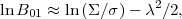 |
(26) |
where as before gives
the number of sigma away from a
null result (the "significance" of the measurement). The first
term on the right-hand-side is approximately the logarithm of
the ratio of the prior to posterior volume. We can interpret it as
the information content of the data, as it gives the factor by
which the parameter space has been reduced in going from the prior
to the posterior. This term is positive for informative data, i.e.
if the likelihood is more sharply peaked than the prior. The
second term is always negative, and it favours the more complex
model if the measurement gives a result many sigma away from the
prediction of the simpler model (i.e., for
≫ 0). We
are free to measure the information content in base-10 logarithm
(as this quantity is closer to our intuition, being the order of
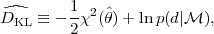
magnitude of our information increase), and we define the quantity
I10  log10(
/ ).
Figure 3 shows contours of |
ln B01
| = const for const = 1.0,2.5,5.0 in the (I10,
)
plane, as computed from Eq. (26). The contours
delimit significative levels for the strength of evidence,
according to the Jeffreys' scale (Table 1). For
moderately informative data (I10 ≈ 1 - 2) the
measured mean has to lie at least about
4 away from 0 in order to
robustly disfavor the simpler model (i.e.,
log10(
/ ).
Figure 3 shows contours of |
ln B01
| = const for const = 1.0,2.5,5.0 in the (I10,
)
plane, as computed from Eq. (26). The contours
delimit significative levels for the strength of evidence,
according to the Jeffreys' scale (Table 1). For
moderately informative data (I10 ≈ 1 - 2) the
measured mean has to lie at least about
4 away from 0 in order to
robustly disfavor the simpler model (i.e.,
 4).
Conversely, for
3 highly informative data (I10
2) do favor the conclusion that the extra parameter is
indeed 0. In general, a large information content favors the
simpler model, because Occam's razor penalizes the large volume of
"wasted" parameter space of the extended model.
4).
Conversely, for
3 highly informative data (I10
2) do favor the conclusion that the extra parameter is
indeed 0. In general, a large information content favors the
simpler model, because Occam's razor penalizes the large volume of
"wasted" parameter space of the extended model.
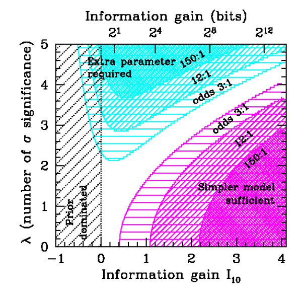 |
Figure 3. Illustration of Bayesian model
comparison for two nested
models, where the more complex model has one extra parameter. The
outcome of the model comparison depends both on the information
content of the data with respect to the a priori available
parameter space, I10 (horizontal axis) and on the
quality of fit(vertical axis,
|
An useful properties of Figure 3 is that the
impact of a change of prior can be easily quantified. A different
choice of prior width (i.e.,
) amounts to a
horizontal
shift across Figure 3, at least
as long as I10 > 0 (i.e., the posterior is
dominated by the likelihood). Picking more restrictive priors
(reflecting more predictive theoretical models) corresponds to shifting
the result of the model comparison to the left of
Figure 3, returning an inconclusive result
(white region) or a prior-dominated outcome (hatched region).
Notice that results in the 2-3 sigma range, which are fairly
typical in cosmology, can only support the more complex model in a
very mild way at best (odds of 3:1 at best), while actually
being most of the time either inconclusive or in favour of the
simpler hypothesis (pink shaded region in the bottom right corner).
Bayesian model comparison is usually conservative when it comes to admitting a new quantity in our model, even in the case when the prior width is chosen incorrectly. Consider the following two possibilities:
In both cases the result of the model comparison will eventually override the "wrong" prior choice (although it might take a long time to do so), exactly as it happens for parameter inference.
4.5. Getting around the prior - The maximal evidence for a new parameter
For nested models, Eq. (23) shows that the
relative probability of the more complex model can be made
arbitrarily small by increasing the broadness of the prior for the
extra parameters, p( |
1) (as the prior
is a pdf, it must integrate to unit probability. Hence a broader prior
corresponds to a smaller value of
p(
| 1) = 0
in the denominator). Often, this is not problematical as prior
ranges for the new parameters can (and should) be motivated from
the underlying theory. For example, in assessing whether the
scalar spectral index (ns) of the primordial perturbations
differs from the scale-invariant value ns = 1, the
prior range of the index can be constrained to be 0.8
ns
1.2 within the theoretical framework of slow roll inflation (more on
this in section 6). The sensitivity
of the model comparison result can also be investigated for other
plausible, physically motivated choices of prior ranges, see e.g.
[59,
60].
If the model comparison
outcome is qualitatively the same for a broad choice of plausible
priors, then we can be confident that the result is robust.
Although the Bayesian evidence offers a well-defined framework for model comparison, there are cases where there is not a specific enough model available to place meaningful limits on the prior ranges of new parameters in a model. This hurdle arises frequently in cases when the new parameters are a phenomenological description of a new effect, only loosely tied to the underlying physics, such as for example expansion coefficients of some series. An interesting possibility in such a case is to choose the prior on the new parameters in such a way as to maximise the probability of the new model, given the data. If, even under this best case scenario, the more complex model is not significantly more probable than the simpler model, then one can confidently say that the data does not support the addition of the new parameters, without worrying that some other choice of prior will make the new model more probable [61 - 63].
Consider the Bayes factor in favour of the more complex model,
B10 1 /
B01, with B01 given by
Eq. (20). The simpler model,
0, is
obtained from 0
by setting =
*. An
absolute upper bound to the evidence in favour of the more complex
model is obtained by choosing
p(|1)
to be a delta function centered at the maximum likelihood value under
1,
max. It can
be shown that in this case the upper bound
B10
corresponds to the likelihood ratio between
max and
*. However,
it can be argued that such a choice for the
prior is unjustified, as it can only be made ex post facto
after one has seen the data and obtained the maximum likelihood
estimate. It is more natural to appeal to a mild principle of
indifference as to the value of the parameter under the more
complex model, and thus to maximize the evidence over priors that
are symmetric about
* and
unimodal. This can be shown
to be equivalent to maximizing over all priors that are uniform
and symmetric about
*. This
procedure leads to a very
simple expression for the lower bound on the Bayes factor
[61]
 |
(27) |
for ℘
e-1, where e is the exponential of
one. Here, ℘ is the p-value, the probability that the
the value of some test statistics be as large as or larger than
the observed value assuming the null hypothesis (i.e., the
simpler model) is true (see
[61,
62]
for a detailed discussion). A more precise definition of p-values is
given in any standard statistical textbook, e.g.
[64].
Eq. (27) offers a useful
calibration of frequentist significance values (p-values) in
terms of upper bounds on the Bayesian evidence in favour of the
extra parameters. The advantage is that the quantity on the
left-hand side of Eq. (27) can
be straightforwardly interpreted as an upper bound on the odds for
the more complex model, whereas the p-values cannot. This point
is illustrated very clearly with an astronomical example in
[66].
In fact, a word of caution is in place regarding the meaning of the
p-value, which is often misinterpreted as an error probability,
i.e. as giving the fraction of wrongly rejected nulls in the long
run. For example, when a frequentist test rejects the null hypothesis
(in our example, that =
*) at the 5%
level, this does not mean that one
will make a mistake roughly 5% of the time if one were to repeat
the test many times. The actual error probability is much larger
than that, and can be shown to be at least 29% (for
unimodal, symmetric priors, see Table 6 in
[62]).
This important conceptual point is discussed in in greater detail in
[62,
63,
67].
The fundamental
reason for this discrepancy with intuition is that frequentist
significance tests give the probability of observing data as
extreme or more extreme than what has actually been measured,
assuming the null hypothesis
 0 to be true (which
in Bayesian terms amounts to the choice of a model,
0). But
the quantity one is interested in is actually the probability of
the model 0
given the observations, which can only be obtained by using Bayes'
Theorem to invert the order of conditioning
5.
Indeed, in frequentist statistics, a hypothesis is either true or false
(although we do not know which case it is) and it is meaningless
to attach to it a probability statement.
0 to be true (which
in Bayesian terms amounts to the choice of a model,
0). But
the quantity one is interested in is actually the probability of
the model 0
given the observations, which can only be obtained by using Bayes'
Theorem to invert the order of conditioning
5.
Indeed, in frequentist statistics, a hypothesis is either true or false
(although we do not know which case it is) and it is meaningless
to attach to it a probability statement.
Table 2 lists B10 for some common thresholds for significance values and the strength of evidence scale, thus giving a conversion table between significance values and upper bounds on the Bayesian evidence, independent of the choice of prior for the extra parameter (within the class of unimodal and symmetric priors). It is apparent that in general the upper bound on the Bayesian evidence is much more conservative than the p-value, e.g. a 99% result (corresponding to ℘ = 0.01) corresponds to odds of 8:1 at best in favour of the extra parameters, which fall short of even the "moderate evidence" threshold. Strong evidence at best requires at least a 3.6 sigma result. A useful rule of thumb is thus to think of a s sigma result as a s-1 sigma result, e.g. a 99.7% result (3 sigma) really corresponds to odds of 21:1, i.e. about 95% probability for the more complex model. Thus when considering the detection of a new parameter, instead of reporting frequentist significance values it is more appropriate to present the upper bound on the Bayes factor, as this represents the maximum probability that the extra parameter is different from its value under the simpler model.
| p-value | B10 | lnB10 | sigma | category |
| 0.05 | 2.5 | 0.9 | 2.0 | |
| 0.04 | 2.9 | 1.0 | 2.1 | `weak' at best |
| 0.01 | 8.0 | 2.1 | 2.6 | |
| 0.006 | 12 | 2.5 | 2.7 | `moderate' at best |
| 0.003 | 21 | 3.0 | 3.0 | |
| 0.001 | 53 | 4.0 | 3.3 | |
| 0.0003 | 150 | 5.0 | 3.6 | `strong' at best |
| 6 × 10⁻⁷ | 43000 | 11 | 5.0 | |
This approach has been applied to the cosmological context in [65], who analysed the evidence in favour of a non-scale invariant spectral index and of asymmetry in the cosmic microwave background maps. For further details on the comparison between frequentist hypothesis testing and Bayesian model selection, see [28].
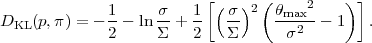
4.6. The effective number of parameters - Bayesian model complexity
The usefulness of a Bayesian model selection approach based on the Bayesian evidence is that it tells us whether the increased "complexity" of a model with more parameters is justified by the data. However, it is desirable to have a more refined definition of "model complexity", as the number of free parameters is not always an adequate description of this concept. For example, if we are trying to measure a periodic signal in a time series, we might have a model of the data that looks like
 |
(28) |
where A,
,
 are free parameters we
wish to
constrain. But if is
very small compared to 1 and the noise is large compared to
, then the oscillatory term
remains unconstrained by the data and effectively we can only
measure the normalization A. Thus the parameters
,
should not count as
free parameters as they cannot be
constrained given the data we have, and the effective model
complexity is closer to 1 than to 3. From this example it follows
that the very notion of "free parameter" is not absolute, but it
depends on both what our expectations are under the model, i.e. on
the prior, and on the constraining power of the data at hand.
are free parameters we
wish to
constrain. But if is
very small compared to 1 and the noise is large compared to
, then the oscillatory term
remains unconstrained by the data and effectively we can only
measure the normalization A. Thus the parameters
,
should not count as
free parameters as they cannot be
constrained given the data we have, and the effective model
complexity is closer to 1 than to 3. From this example it follows
that the very notion of "free parameter" is not absolute, but it
depends on both what our expectations are under the model, i.e. on
the prior, and on the constraining power of the data at hand.
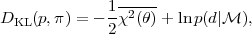
In order to define a more appropriate measure of complexity, in
[68]
the notion of Bayesian
complexity was introduced, which measures the number of
parameters that the data can support. Consider the information
gain obtained when upgrading the prior to the posterior, as
measured by the the Kullback-Leibler (KL) divergence
[69]
between the posterior, p and the prior, denoted here by
 :
:
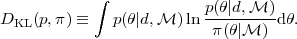 |
(29) |
In virtue of Bayes' theorem,
p(|d,
) =
()
( | ) / p(d |
) hence the KL
divergence becomes the sum of the negative log evidence and the
expectation value of the log-likelihood under the posterior:
 |
(30) |
To gain a feeling for what the KL divergence expresses, let us
compute it for a 1-dimensional case, with a Gaussian prior around
0 of variance
2 and a
Gaussian likelihood centered on
max and variance
2. We obtain
after a short calculation
 |
(31) |
The second term on the right-hand side gives the reduction in
parameter space volume in going from the prior to the posterior.
For informative data,
/ ≪ 1, this
terms is positive and grows as the logarithm of the volume ratio. On the
other hand, in the same regime the third term is small unless the
maximum likelihood estimate is many standard deviations away from
what we expected under the prior, i.e. for
max /
≫ 1.
This means that the maximum likelihood value is "surprising", in
that it is far from what our prior led us to expect. Therefore we
can see that the KL divergence is a summary of the amount of
information, or "surprise", contained in the data.
Let us now define an effective
 2 through the
likelihood as
()
= exp(-2 / 2).
Then Eq. (30) gives
2 through the
likelihood as
()
= exp(-2 / 2).
Then Eq. (30) gives
 |
(32) |
where the bar indicates a mean taken over the posterior distribution. The posterior average of the effective chi-square is a quantity can be easily obtained by Markov chain Monte Carlo techniques (see section 3.2). We then subtract from the "expected surprise" the estimated surprise in the data after we have actually fitted the model parameters, denoted by
 |
(33) |
where the first term on the right-hand-side is the effective chi-square at the estimated value of the parameters, indicated by a hat. This will usually be the posterior mean of the parameters, but other possible estimators are the maximum likelihood point or the posterior median, depending on the details of the problem. We then define the quantity
 |
(34) |
(notice that the evidence term is the same in
Eqs. (32) and (33) as it
does not depend on the parameters and therefore it disappears from
the complexity). The Bayesian complexity gives the effective
number of parameters as a measure of the constraining power
of the data as compared to the predictivity of the model,
i.e. the prior. Hence
 b depends both
on the data and on the prior available parameter space. This can be
understood by considering further the toy example of a Gaussian
likelihood of variance
2 around
max and a
Gaussian prior around 0 of variance
2. Then a
short calculation shows that the Bayesian complexity is given by (see
[70]
for details)
b depends both
on the data and on the prior available parameter space. This can be
understood by considering further the toy example of a Gaussian
likelihood of variance
2 around
max and a
Gaussian prior around 0 of variance
2. Then a
short calculation shows that the Bayesian complexity is given by (see
[70]
for details)
 |
(35) |
So for /
≪ 1,
b ≈ 1 and
the model has one effective, well constrained parameter. But if the
likelihood width is large compared to the prior,
/
≫ 1, then the experiment is not informative with respect to our
prior beliefs and
b → 0.
The Bayesian complexity can be a useful diagnostic tool in the
tricky situation where the evidence for two competing models is
about the same. Since the evidence does not penalize parameters
that are unmeasured, from the evidence alone we cannot know if we
are in the situation where the extra parameters are simply
unconstrained and hence irrelevant
( ≪ 1 in the example
of Eq. (28)) or if they improve the
quality-of-fit just enough to offset the Occam's razor penalty
term, hence giving the same evidence as the simpler model. The
Bayesian complexity breaks this degeneracy in the evidence
allowing to distinguish between the two cases:
0)
≈ p(d|
1) and
b(1) >
b(0):
the quality of the data is sufficient to measure the additional
parameters of the more complicated model
(1), but they do
not improve its evidence by much. We should prefer model
0,
with less parameters.
0)
≈ p(d
| 1) and
b(1)
≈ b(0):
both models have a comparable evidence and the effective
number of parameters is about the same. In this case the data is
not good enough to measure the additional parameters of the more
complicated model (given the choice of prior) and we cannot draw
any conclusions as to whether the extra parameter is needed.The first application of this technique in the cosmological context is in [70], where it is applied to the number of effective parameters from cosmic microwave background data, while in [71] it was used to determine the number of effective dark energy parameters.
4.7. Information criteria for approximate model comparison
Sometimes it might be useful to employ methods that aim at an approximate model selection under some simplifying assumptions that give a default penalty term for more complex models, which replaces the Occam's razor term coming from the different prior volumes in the Bayesian evidence. While this is an obviously appealing feature, on closer examination it has the drawback of being meaningful only in fairly specific cases, which are not always met in astrophysical or cosmological applications. In particular, it can be argued that the Bayesian evidence (ideally coupled with an analysis of the Bayesian complexity) ought to be preferred for model building since it is precisely the lack of predictivity of more complicated models, as embodied in the physically motivated range of the prior, that ought to penalize them.
With this caveat in mind, we list below three types of information criteria that have been widely used in several astrophysical and cosmological contexts. An introduction to the information criteria geared for astrophysicists is given by Ref. [72]. A discussion of the differences between the different information criteria as applied to astrophysics can be found in [73], which also presents a few other information criteria not discussed here.
 |
(36) |
where max
p(d |
max,
) is the maximum
likelihood value. The derivation of the AIC follows from an
approximate minimization of the KL divergence between the true
model distribution and the distribution being fitted to the data.
 |
(37) |
where k is the number of fitted parameters as before and N is the number of data points. The best model is again the one that minimizes the BIC.
 |
(38) |
In this form, the DIC is reminiscent of the AIC, with the ln
max term
replaced by the estimated KL divergence and the number
of free parameters by the effective number of parameters,
b,
from Eq. (34). Indeed, in the limit of
well-constrained parameters, the AIC is recovered
from (38), but the DIC has the advantage of
accounting for unconstrained directions in parameters space.
The information criteria ought to be interpreted with care when applied to real situations. Comparison of Eq. (37) with Eq. (36) shows that for N > 7 the BIC penalizes models with more free parameters more harshly than the AIC. Furthermore, both criteria penalize extra parameters regardless of whether they are constrained by the data or not, unlike the Bayesian evidence. This comes about because implicitly both criteria assume a "data dominated" regime, where all free parameters are well constrained. But in general the number of free parameters might not be a good representation of the actual number of effective parameters, as discussed in section 4.6. In a Bayesian sense it therefore appears desirable to replace the number of parameters k by the effective number of parameters as measured by the Bayesian complexity, as in the DIC.
It is instructive to inspect briefly the derivation of the BIC.
The unnormalized posterior
g()
()
p(|) can be
approximated by a multi-variate Gaussian
around its mode ,
i.e. g() ≈
g() - 1/2
( -
)t
F ( -
), where
F is minus the Hessian of the posterior evaluated at the
posterior mode. Then the evidence integral can be computed analytically,
giving
 |
(39) |
For large samples, N → ∞, the posterior mode
tends to the maximum likelihood point,
→
max, hence
g()
→ max
p(max)
and the log-evidence becomes
 |
(40) |
where the error introduced by the various approximations scales to
leading order as
 (N-1/2).
On the right-hand-side, the first term scales as
(N), the second and
third terms are
constant in N, while the last term is given by ln| F
| ≈ k lnN, since the variance scales as the number of
data points, N. Dropping terms of order
(1) or
below
6,
we obtain
(N-1/2).
On the right-hand-side, the first term scales as
(N), the second and
third terms are
constant in N, while the last term is given by ln| F
| ≈ k lnN, since the variance scales as the number of
data points, N. Dropping terms of order
(1) or
below
6,
we obtain
 |
(41) |
Thus maximising the evidence of Eq. (41) is
equivalent to minimizing the BIC in Eq. (37). We see
that dropping the term
lnp(max)
in (40)
means that effectively we expect to be in a regime where the model
comparison is dominated by the likelihood, and that the prior
Occam's razor effect becomes negligible. This is often not the
case in cosmology. Furthermore, this "weak" prior choice is
intrinsic (even though hidden from the user) in the form of the
BIC, and often it is not justified. In conclusion, it appears that
what makes the information criteria attractive, namely the absence
of an explicit prior specification, represents also their
intrinsic limitation.
3 In its formulation by the medieval English philosopher and Franciscan monk William of Ockham (ca. 1285-1349): "Pluralitas non est ponenda sine neccesitate". Back.
4 Publicly available modules implementing nested sampling can be found at cosmonest.org [51] and http://www.mrao.cam.ac.uk/software/cosmoclust/ [52] (accessed Feb 2008). Back.
5 To convince oneself of the difference between the two quantities, consider the following example [22]. Imagine selecting a person at random — the person can either be male or female (our hypothesis). If the person is female, her probability of being pregnant (our data) is about 3%, i.e. p(pregnant|female) = 0.03. However, if the person is pregnant, her probability of being female is much larger than that, i.e. (female|pregnant)≫ 0.03. The two conditional probabilities are related by Bayes' theorem. Back.
6 See [76] for a more careful treatment, where a better approximation is obtained by assuming a weak prior which contains the same information as a single datum. Back.