


Driven by the emergence of inexpensive sensors and computing capabilities, the amount of cosmological data has been increasing exponentially over the last 15 years or so. For example, the first map of cosmic microwave background (CMB) anisotropies obtained in 1992 by COBE [77] contained ~ 103 pixels, which became ~ 5 × 104 by 2002 with CBI [78, 79]. Current state-of-the art maps (from the WMAP satellite [80]) involve ~ 106 pixels, which are set to grow to ~ 107 with Planck in the next couple of years. Similarly, angular galaxy surveys contained ~ 106 objects in the 1970's, while by 2005 the Sloan Digital Sky Survey [81] had measured ~ 2 × 10⁸ objects, which will increase to ~ 3 × 109 by 2012 when the Large Synoptic Survey Telescope [82] comes online 7.
This data explosion drove the adoption of more efficient map making tools, faster component separation algorithms and parameter inference methods that would scale more favourably with the number of dimensions of the problem. As data sets have become larger and more precise, so has grown the complexity of the models being used to describe them. For example, if only 2 parameters could meaningfully be extracted from the COBE measurement of the large-scale CMB temperature power spectrum (namely the normalization and the spectral tilt [77, 83]), the number of model parameters had grown to 11 by 2002, when smaller-scale measurements of the acoustic peaks had become available. Nowadays, parameter spaces of up to 20 dimensions are routinely considered.
This section gives an introduction to the broad problem of cosmological parameter inference and highlights some of the tools that have been introduced to tackle it, with particular emphasis on innovative techniques. This is a vast field and any summary is bound to be only sketchy. We give throughout references to selected papers covering both historically important milestones and recent major developments.
5.1. The "vanilla"
 CDM cosmological
model
CDM cosmological
model
Before discussing the quantities we are interested in measuring in
cosmology (the "cosmological parameters") and some of the
observational probes available to do so, we briefly sketch the
general framework which goes under the name of "cosmological
concordance model". Because it is a relatively simple scenario
containing both a cosmological constant
() and cold dark
matter (CDM) (more about them below), it is also known as the
"vanilla" CDM model.
Our current cosmological picture is based on the scenario of an expanding Universe, as implied by the observed redshift of the spectra of distant galaxies (Hubble's law). This in turn means that the Universe began from a hot and dense state, the initial singularity of the Big Bang. The existence of the cosmic microwave background lends strong support to this idea, as it is interpreted as the relic radiation from the hotter and denser primordial era. The expanding spacetime is described by Einstein's general relativity. The cosmological principle states that the Universe is isotropic (i.e., the same in all directions) and homogeneous (the same everywhere). If follows that an isotropically expanding Universe is described by the so-called Friedmann-Robertson-Walker metric,
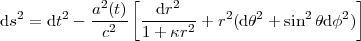 |
(42) |
where  defines the
geometry of spatial sections (if
is positive, the
geometry is spherical; if it is zero,
the geometry is flat; if it is negative, the geometry is
hyperbolic). The scale factor a(t) describes the
expansion of the Universe, and it is related to redshift z by
defines the
geometry of spatial sections (if
is positive, the
geometry is spherical; if it is zero,
the geometry is flat; if it is negative, the geometry is
hyperbolic). The scale factor a(t) describes the
expansion of the Universe, and it is related to redshift z by
 |
(43) |
where a(t0) is the scale factor today and a(t) the scale factor at redshift z. The relation between redshift and comoving distance r is obtained from the above metric via the Friedmann equation, and is given by
 |
(44) |
where H0 is the Hubble constant, and
 x are the
cosmological parameters describing the matter-energy
content of the Universe. Standard parameters included in the
vanilla model are neutrinos
(
x are the
cosmological parameters describing the matter-energy
content of the Universe. Standard parameters included in the
vanilla model are neutrinos
( , with a mass
 1 eV), photons
(
1 eV), photons
( ),
baryons (b),
cold dark matter
(cdm) and
a cosmological constant
(). The curvature
term
is included
for completeness but is currently not required by the standard
cosmological model (see section 6).
The comoving distance determines the apparent brightness of
objects, their apparent size on the sky and the number density of
objects in a comoving volume. Hence measurements of the brightness
of standard candles, of the length of standard rulers or of the
number density of objects at a given redshift leads to the
determination of the cosmological parameters in
Eq. (44) (see next section).
),
baryons (b),
cold dark matter
(cdm) and
a cosmological constant
(). The curvature
term
is included
for completeness but is currently not required by the standard
cosmological model (see section 6).
The comoving distance determines the apparent brightness of
objects, their apparent size on the sky and the number density of
objects in a comoving volume. Hence measurements of the brightness
of standard candles, of the length of standard rulers or of the
number density of objects at a given redshift leads to the
determination of the cosmological parameters in
Eq. (44) (see next section).
The currently accepted paradigm for the generation of density fluctuations in the early Universe is inflation. The idea is that quantum fluctuations in the primordial era were stretched to cosmological scales by an initial period of exponential expansion, called "inflation", possibly driven by a yet unknown scalar field. This increased the scale factor by about 26 orders of magnitude within about 10-32s after the Big Bang. Although presently we have only indirect evidence for inflation, it is commonly accepted that such a short burst of exponential growth in the scale factor is required to solve the horizon problem, i.e. to explain why the CMB is so highly homogeneous across the whole sky. The quantum fluctuations also originated temperature anisotropies in the CMB, whose study has proved to be one of the powerhouses of precision cosmology. From the initial state with small perturbations imprinted on a broadly uniform background, gravitational attraction generated the complex structures we see in the modern Universe, as indicated both by observational evidence and highly sophisticated computer modelling.
Of course it is possible to consider completely different models,
based for example on alternative theories of gravity (such as
Bekenstein's theory
[84,
85]
or Jordan-Brans-Dicke theory
[86]),
or on a different way of comparing model predictions with
observations
[87 -
89].
Discriminating among models and determining which model is in best
agreement with the data is a task for model comparison techniques,
whose application to cosmology is discussed
section 6. Here we will take the
vanilla CDM model
as our starting point for the following
considerations on cosmological parameters and how they are measured.
5.2. Cosmological observations
The discovery of temperature fluctuations in the Cosmic Microwave Background (CMB) in 1992 by the COBE satellite [77] marked the beginning of the era of precision cosmology. Many other observations have contributed to the impressive development of the field in less than 20 years. For example, around 1990 the picture of flat Universe with both cold dark matter and a positive cosmological constant was only beginning to emerge, and only thanks to the painstakingly difficult work of gluing together several fairly indirect clues [90]. At the time of writing (January 2008), the total density is known with an error of order 1%, and it is likely that this uncertainty will be reduced by another two orders of magnitude in the mid-term [91]. The high accuracy of modern precision cosmology rests on the combination of several different probes, that constrain the physical properties of the Universe at many different redshifts.
 T /
T ~ 10-5) and hence linear perturbation theory
is mostly sufficient to predict very accurately their statistical
distribution. The 2-point correlation function of the
anisotropies is usually described via its Fourier transform, the
angular power spectrum, which presents a series of
characteristic peaks called acoustic oscillations, see e.g.
[92,
93].
Their structure depends in a rich way on the cosmological parameters
introduced in Eq. (44), as well as on the initial
conditions for the perturbations emerging from the inflationary
era (see e.g.
[94,
95,
96]
for further details). The anisotropies are polarized at the level of
1%, and measuring accurately the information encoded by the weak
polarization signal is the goal of many ongoing observations.
State-of-the art measurements are described in e.g.
[80,
97,
98,
99,
100,
101].
An example of recent measurements of the temperature power
spectrum is shown in Figure 4. Later this year, the
Planck satellite is expected to start full-sky, high-resolution
observations of both temperature and polarization.
T /
T ~ 10-5) and hence linear perturbation theory
is mostly sufficient to predict very accurately their statistical
distribution. The 2-point correlation function of the
anisotropies is usually described via its Fourier transform, the
angular power spectrum, which presents a series of
characteristic peaks called acoustic oscillations, see e.g.
[92,
93].
Their structure depends in a rich way on the cosmological parameters
introduced in Eq. (44), as well as on the initial
conditions for the perturbations emerging from the inflationary
era (see e.g.
[94,
95,
96]
for further details). The anisotropies are polarized at the level of
1%, and measuring accurately the information encoded by the weak
polarization signal is the goal of many ongoing observations.
State-of-the art measurements are described in e.g.
[80,
97,
98,
99,
100,
101].
An example of recent measurements of the temperature power
spectrum is shown in Figure 4. Later this year, the
Planck satellite is expected to start full-sky, high-resolution
observations of both temperature and polarization.
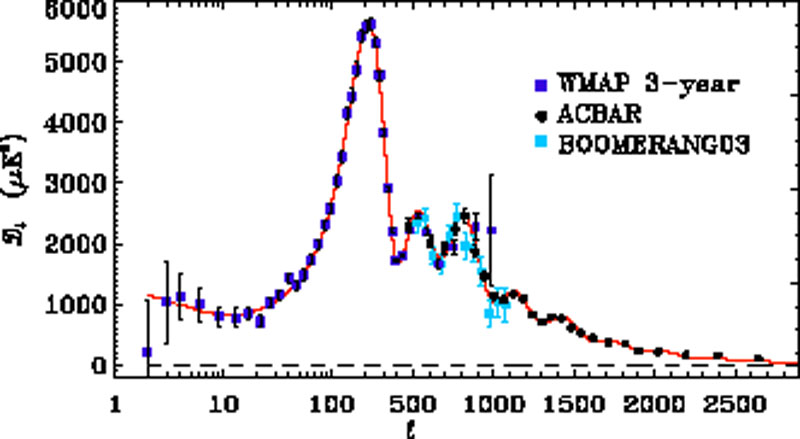 |
Figure 4. State-of-the-art cosmic microwave
background temperature power spectrum measurements along with the best-fit
|
 forest
[102],
although concerns remain about the reliability of the theoretical
modelling of non-linear effects. Recently, both the Sloan Digital Sky
Survey
[103]
and the 2dF Galaxy Redshift Survey
[104]
have detected the presence of baryonic acoustic oscillations,
which appear as a bump in the
galaxy-galaxy correlation function corresponding to the scale of
the acoustic oscillations in the CMB. The physical meaning is that
galaxies tend to form preferentially at a separation corresponding
to the characteristic scale of inhomogeneities in the CMB.
Baryonic oscillations can be used as rulers of known length
(measured via the CMB acoustic peaks) located at a much smaller
redshift than the CMB (currently, z ~ 0.3), and hence they are
powerful probes of the recent expansion history of the Universe,
with particular focus on dark energy properties. The distribution
of clusters with redshift can also be employed to probe the growth
of perturbations and hence to constrain cosmology. Current galaxy
redshift surveys have catalogued about half a million objects, but
a new generation of surveys aims at taking this number to a over a
billion.
forest
[102],
although concerns remain about the reliability of the theoretical
modelling of non-linear effects. Recently, both the Sloan Digital Sky
Survey
[103]
and the 2dF Galaxy Redshift Survey
[104]
have detected the presence of baryonic acoustic oscillations,
which appear as a bump in the
galaxy-galaxy correlation function corresponding to the scale of
the acoustic oscillations in the CMB. The physical meaning is that
galaxies tend to form preferentially at a separation corresponding
to the characteristic scale of inhomogeneities in the CMB.
Baryonic oscillations can be used as rulers of known length
(measured via the CMB acoustic peaks) located at a much smaller
redshift than the CMB (currently, z ~ 0.3), and hence they are
powerful probes of the recent expansion history of the Universe,
with particular focus on dark energy properties. The distribution
of clusters with redshift can also be employed to probe the growth
of perturbations and hence to constrain cosmology. Current galaxy
redshift surveys have catalogued about half a million objects, but
a new generation of surveys aims at taking this number to a over a
billion.
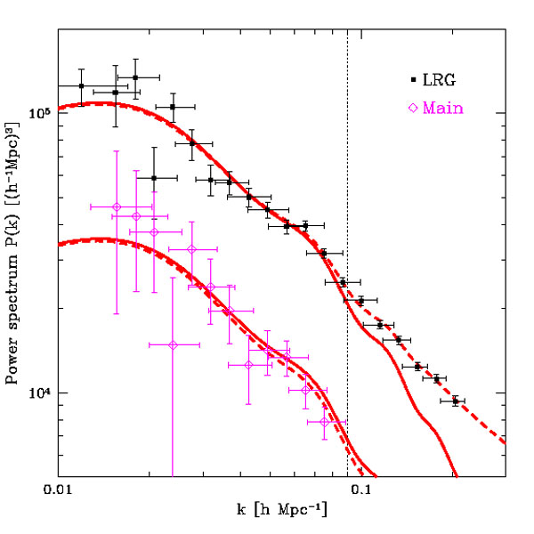 |
Figure 5. Current matter power spectrum
measurements from the Sloan Digital Sky Survey and best-fit
|
5.3. Constraining cosmological parameters
As outlined is section 3.1, our inference problem is fully specified once we give the model (which parameters are allowed to vary and their prior distribution) and the likelihood function for the data sets under consideration. For the cosmological observations described above, relevant cosmological parameters can be broadly classified in four categories.
 crit
= 1.88 × 10⁻²⁹ h2 g/cm3. The
remaining density parameters
(x in
Eq. (44)) are then
written in units of the critical energy density, so that for
example the energy density in baryons is given by
b =
b
crit.
Standard parameters include the energy density in photons
(),
neutrinos
(), baryons
(b),
cold dark matter
(cdm),
cosmological constant
() or, more
generally, a possibly time-dependent dark energy
(de).
crit
= 1.88 × 10⁻²⁹ h2 g/cm3. The
remaining density parameters
(x in
Eq. (44)) are then
written in units of the critical energy density, so that for
example the energy density in baryons is given by
b =
b
crit.
Standard parameters include the energy density in photons
(),
neutrinos
(), baryons
(b),
cold dark matter
(cdm),
cosmological constant
() or, more
generally, a possibly time-dependent dark energy
(de).
5.3.1. The joint likelihood function.
When the observations are independent, the log-likelihoods for
each observation simply add
8.
Defining  2
2
 -2
ln
-2
ln , we have that
 |
(45) |
One important advantage of combining different observations as in Eq. (45) is that each observable has different degenerate directions, i.e. directions in parameter space that are poorly constrained by the data. By combining two or more types of observables, it is often the case that the two data sets together have a much stronger constraining power than each one of them separately, because they mutually break parameters degeneracies. Combination of data sets should never be carried out blindly, however. The danger is that the data sets might be mutually inconsistent, in which case combining them singles out in the posterior a region that is not favoured by any of the two data sets separately, which is obviously unsatisfactory. Such discrepancies might arise because of undetected systematics, or insufficient modelling of the observations.
In order to account for possible discrepancies of this kind, Ref. [122] suggested to replace Eq. (45) by
 |
(46) |
where i are
(unknown) weight factors
("hyperparameters") for the various data sets, which determine
the relative importance of the observations. A non-informative
prior is specified for the hyperparameters, which are then
integrated out in a Bayesian way, obtaining an effective
chi-square
 |
(47) |
where Ni is the number of data points in data set i. This method has been applied to combine different CMB observations in the pre-WMAP era [122, 123]. A technique based on the comparison of the Bayesian evidence for different data sets has been employed in [124], while Ref. [125] uses a technique similar in spirit to the hyperparameter approach outlined above to perform a binning of mutually inconsistent observations suffering from undetected systematics, as explained in [126].
After the likelihood has been specified, it remains to work out the posterior pdf, usually obtained numerically via MCMC technology, and report posterior constraints on the model parameters, e.g. by plotting 1 or 2-dimensional posterior contours. We now sketch the way this program has been carried out as far as cosmological parameter estimation is concerned.
5.3.2. Likelihood-based parameter
determination.
Up until around 2002, the method of choice for cosmological
parameter estimation was either direct numerical maximum
likelihood search
[127,
128]
or evaluation of the likelihood on a grid in parameter space. Once
the likelihood has been mapped out, (frequentist) confidence
intervals for the parameters are obtained by finding the
maximum-likelihood point (or, equivalently, the minimum
chi-square) and by delimiting the region of parameter space where
the log-likelihood drops by a specified amount (details can be
found in any standard statistics textbook). If the likelihood is a
multi-normal Gaussian, then this procedure leads to the familiar
"delta chi-square" rule-of-thumb, i.e. that e.g. a 95.4%
(2  ) confidence interval
for 1 parameter is delimited by the region where the
2
-2
log increases by
2
= 4.00 from its minimum value (see e.g.
[43]).
Of course the value of
2
depends both on the number of parameters being constrained and on
the desired confidence interval
9.
) confidence interval
for 1 parameter is delimited by the region where the
2
-2
log increases by
2
= 4.00 from its minimum value (see e.g.
[43]).
Of course the value of
2
depends both on the number of parameters being constrained and on
the desired confidence interval
9.
Approximate confidence intervals for each parameter were then usually obtained from the above procedure, after maximising the likelihood across the hidden dimensions rather than marginalising [130, 131], since the latter procedure required a computationally expensive multi-dimensional integration. The rationale was that maximisation is approximately equivalent to marginalisation for close-to-Gaussian problems (a simple proof can be found in Appendix A of [132]), although it was early recognized that this is not always a good approximation for real-life situations [133]. Marginalisation methods based on multi-dimensional interpolation were devised and applied in order to improve on this respect [132, 134]. Many studies adopted this methodology, which could not quite be described as fully Bayesian yet since it was likelihood-based and the the notion of posterior was not explicitly introduced. Often, the choice of particular theoretical scenarios (for example, a flat Universe or adiabatic initial conditions) or the inclusion of external constraints (such as bounds on the baryonic density coming from Big Bang nucleosyhntesis) were described as "priors". A more rigorous terminology would call the former a model choice, while the latter amounts to inclusion (in the likelihood) of external information. Since the likelihood could be well approximated by a simple log-normal distribution, its computation cost was fairly low. With the advent of CMBFAST [135], the availability of a fast numerical code for the computation of CMB and matter power spectra meant that grids of up to 30 million points and parameter spaces of dimensionality up to order 10 could be handled in this way [134].
5.3.3. Bayes in the sky — The rise of
MCMC.
The watershed moment after which methods based on likelihood
evaluation on a grid where definitely overcome by Bayesian MCMC
methods can perhaps be indicated in Ref.
[136],
which marked one of the last major studies performed using
essentially frequentist techniques. Pioneering works in using MCMC
technology for cosmological parameter extraction include the
application to VSA data
[137,
45],
the use of simulated annealing
[138]
and the study of Ref.
[139].
But it was the release of the CosmoMC code
10
in 2002
[140]
that made a huge impact on the
cosmological community, as CosmoMC quickly became a standard and
user-friendly tool for Bayesian parameter inference from CMB,
large scale structure and other data. The favourable scalability
of MCMC methods with dimensionality of the parameter space and the
easiness of marginalization were immediately recognized as major
advantages of the method. CosmoMC employs the CAMB
code
[141]
to compute the matter and CMB power
spectra from the physical model parameters. It then employs
various MCMC algorithms to sample from the posterior distribution
given current CMB, matter power spectrum (galaxy power spectrum,
baryonic acoustic wiggles and
Lyman- observations) and
supernovae data.
State-of-the-art applications of cosmological parameter
inference can be found in papers such as
[105,
142,
143,
97].
Table 3 summarizes recent posterior credible
intervals on the parameters of the vanilla
CDM model introduced
above while Figure 6 shows the full 1-D
posterior pdf for 6 relevant parameters (both from Ref.
[105]).
The initial conditions emerging from
inflation are well described by one adiabatic degree of freedom
and a distribution of fluctuations that deviates slightly from
scale invariance, but which is otherwise fairly featureless.
| Parameter | Value | Meaning | Definition |
| Matter budget parameters | |||
 s s |
0.5918- 0.0020+ 0.0020 | CMB acoustic angular scale fit (degrees) | s =
rs(zrec) /
dA(zrec) × 180 /
 |
| b |
0.0222- 0.0007+ 0.0007 | Baryon density | b =
b
h2
≈
b
/ (1.88 × 10⁻²⁶kg/m3) |
| c |
0.1050- 0.0040+ 0.0041 | Cold dark matter density | c =
cdm
h2 ≈
c
/ (1.88 × 10⁻²⁶kg/m3) |
| Initial conditions parameters | |||
| As | 0.690- 0.044+ 0.045 | Scalar fluctuation amplitude | Primordial scalar power at k = 0.05/Mpc |
| ns | 0.953- 0.016+ 0.016 | Scalar spectral index | Primordial spectral index at k = 0.05/Mpc |
| Reionization history (abrupt reionization) | |||
 |
0.087- 0.030+ 0.028 | Reionization optical depth | |
| Nuisance parameters (for galaxy power spectrum) | |||
| b | 1.896- 0.069+ 0.074 | Galaxy bias factor | See [105] for details. |
| Qnl | 30.3- 4.1+ 4.4 | Nonlinear correction parameter | See [105] for details. |
| Derived parameters (functions of those above) | |||
| tot |
1.00 (flat Universe assumed) | Total density/critical density | tot =
m +
=
1 -
|
| h | 0.730- 0.019+ 0.019 | Hubble parameter | h =
[(b
+ c ) /
(tot
- )]1/2 |
| b |
0.0416- 0.0018+ 0.0019 | Baryon density/critical density | b
= b /
h2 |
| c |
0.197- 0.015+ 0.016 | CDM density/critical density | cdm
= c /
h2 |
| m |
0.239- 0.017+ 0.018 | Matter density/critical density | m
= b +
cdm |
|
0.761- 0.018+ 0.017 | Cosmological constant density/critical density |
≈ h-2
(1.88
× 10-26kg/m3) |
| 8 |
0.756- 0.035+ 0.035 | Density fluctuation amplitude | See [105] for details. |
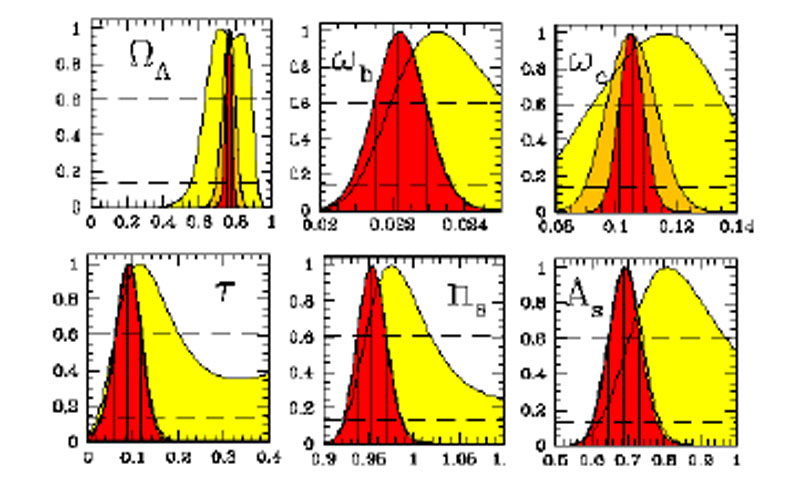 |
Figure 6. Posterior constraints on key cosmological parameters from recent CMB and large scale structure data, compare Table 3. Top row, from left to right, posterior pdf (normalized to the peak) for the cosmological constant density in units of the critical density, the (physical) baryons and cold dark matter densities. Bottom row, from left to right: optical depth to reionization, scalar tilt and scalar fluctuations amplitude. Yellow using WMAP 1-yr data, orange WMAP 3-yr data and red adding Sloan Digital Sky Survey galaxy distribution data. Spatial flatness and adiabatic initial conditions have been assumed. This set of only 6 parameters (plus 2 other nuisance parameters not shown here) appear currently sufficient to describe most cosmological observations (adapted from [105]). |
Addition of extra parameters to this basic description (for example, a curvature term, or a time-evolution of the cosmological constant, in which case it is generically called "dark energy") is best discussed in terms of model comparison rather than parameter inference (see next section). The breath and range of studies aiming at constraining extra parameters is such that it would be impossible to give even a rough sketch here. However we can say that the simple model described by the 6 cosmological parameters given in Table 3 appears at the moment appropriate and sufficient to explain most of the presently available data. MCMC is nowadays almost universally employed in one form or another in the cosmology community.
5.3.4. Recent developments in parameter inference. Nowadays, the likelihood evaluation step is becoming the bottleneck of cosmological parameter inference, as the WMAP likelihood code [80] requires the evaluation of fairly complex correlation terms, while the computational time for the actual model prediction in terms of power spectra is subdominant (except for spatially curved models or non-standard scenarios containing active seeds, such as cosmic strings). This trend is likely to become stronger with future CMB datasets, such as Planck. Currently, for relatively straightforward extensions of the concordance model presented in Table 3, a Markov chain with enough samples to give good inference can be obtained in a couple of days of computing time on a "off-the-shelf" machine with 4 CPUs.
Massive savings in computational effort can be obtained by employing neural networks techniques, a computational methodology consistent of a network of processors called "neurons". Neural networks learn in an unsupervised fashion the structure of the computation to be performed (for example, likelihood evaluation across the cosmological parameter space) from a training set provided by the user. Once trained, the network becomes a fast and efficient interpolation algorithm for new points in the parameter space, or for classification purposes (for example to determine the redshift of galaxies from photometric data [144, 145]). When applied to the problem of cosmological parameter inference, neural networks can teach themselves the structure of the parameter space (for models up to about 10 dimensions) by employing as little as a few thousands training points, for which the likelihood has to be computed numerically as usual. Once trained, the network can then interpolate extremely fast between samples to deliver a complete Markov chain within a few minutes. The speed-up can thus reach a factor of 30 or more [146, 147]. Another promising tool is a machine-learning based algorithm called PICO [148, 149] 11, requiring a training set of order ~ 104 samples, which are then used to perform an interpolation of the likelihood across parameter space. This procedure can achieve a speed-up of over a factor of 1000 with respect to conventional MCMC.
The forefront of Bayesian parameter extraction is quickly moving
on to tackle even more ambitious problems, involving thousands of
parameters. This is the case for the Gibbs sampling technique to
extract the full posterior probability distribution for the power
spectrum Cℓ's directly from CMB maps, performing
component separations (i.e., multi-frequency foregrounds removal) at the
same time and fully propagating uncertainties to the level of
cosmological parameters
[150,
153].
This method has been tested up to ℓ
50 on WMAP
temperature data and is expected to perform well up to ℓ
100-200 for Planck-quality data. Equally impressive is the
Hamiltonian sampling approach
[154],
which returns the Cℓ's posterior pdf from a
(previously foreground
subtracted) CMB map. At WMAP resolution, this involves working
with ~ 105 parameters, but the efficiency is such that the
800 Cℓ distributions (for the temperature signal)
can be obtained in about a day of computation on a high-end desktop
computer.
Another frontier of Bayesian methods is represented by high energy particle physics, which for historical and methodological reasons has been so far mostly dominated by frequentist techniques. However, the Bayesian approach to parameter inference for supersymmetric theories is rapidly gathering momentum, due to its superior handling of nuisance parameters, marginalization and inclusion of all sources of uncertainty. The use of Bayesian MCMC for supersymmetry parameter extraction has been first advocated in [155], and has then been rigorously applied to a detailed analysis of the Constrained Minimal Supersymmetric Standard Model [156 - 161], a problem that involves order 10 free parameters. A public code called SuperBayeS is available to perform an MCMC Bayesian analysis of supersymmetric models 12. Presently, there are hints that the constraining power of the data is insufficient to override the prior choice in this context [162], but future observations, most notably by the Tevatron or LHC [163, 164] and tighter limits (or a detection) on the neutralino scattering cross section [159], should considerably improve the situation in this respect.
5.4. Caveats and common pitfalls
Although Bayesian inference is quickly maturing to become an almost automated procedure, we should not forget that a "black box" approach to the problem always hides dangers and pitfalls. Every real world problem presents its own peculiarities that demand careful consideration and statistical inference remains very much a craft as much as a science. While Bayes' Theorem is never wrong, incorrect specification of the prior (for example, making unwarranted assumptions of failing to specify relevant external information) or inappropriate construction of the likelihood (e.g., not reflecting the experiment or neglecting relevant sources of uncertainty) will easily lead to wrong inferences. Below we list a few common pitfalls that need to be considered in the cosmological context.
a prior which is flat
in ln ("Jeffreys'
prior") is instead the appropriate choice (see e.g.
[6]).
When considering extensions of the
CDM
model, for example, it is common practice to parameterize the new
physics with a set of quantities about which very little (if
anything at all) is known a priori. Assuming flat priors on
those parameters is often an unwarranted choice. Flat priors in
"fundamental" parameters will in general not correspond to a
flat distribution for the observable quantities that are derived
from those parameters, nor for other quantities we might be
interested in constraining. Hence the apparently non-informative
choice for the fundamental parameters is actually highly
informative for other quantities that appear directly in the
likelihood. It is extremely important that this "hidden prior
information" be brought to light, or one could mistake the effect
of the prior for constraining power of the data. An effective way
to do that is to plot pdf's for the quantities of interest without
including the data, i.e. run an MCMC sampling from the prior only (see
[45]
for an instructive example).
7 Alex Szalay, talk at the specialist discussion meeting "Statistical challenges in cosmology and astroparticle physics", held at the Royal Astronomical Society, London, Oct 2007. Back.
8 This is of course not the case when one is carrying out correlation studies, where the aim is precisely to exploit correlation among different observables (for example, the late Integrated Sachs-Wolfe effect). Back.
9 An important technical point is that frequentist confidence intervals are considered random variables — they give the range within which our estimate of the parameter value will fall e.g. 95.4% of the time if we repeat our measurement N→ ∞ times. The true value of the parameter is given (although unknown to us) and has no probability statement attached to it. On the contrary, Bayesian credible intervals containing for example 95.4% of the posterior probability mass represent our degree of belief about the value of the parameter itself. Often, Bayesian credible intervals are imprecisely called "confidence intervals" (a term that should be reserved for the frequentist quantity), thus fostering confusion between the two. Perhaps this happens because for Gaussian cases the two results are formally identical, although their interpretation is profoundly different. This can have important consequences if the true value is near the boundary of the parameter space, in which case the results from the frequentist and Bayesian procedure may differ substantially - see [129] for an interesting example involving the determination of neutrino masses. Back.
10 Available from: cosmologist.info/cosmomc (accessed Jan 20th 2008). Back.
11 Available from: http://cosmos.astro.illinois.edu/pico/ (accessed Jan 14th 2008). Back.
12 Code available from: superbayes.org (accessed Feb 13th 2008). Back.