


Stellar mass is one of the most important and useful quantities that can be estimated for a high-redshift galaxy. There are two reasons for this. First, since it represents the time-integral of past star-formation activity, it can be compared directly with observed star-formation rates in even higher-redshift galaxies to set model-independent constraints on plausible modes of galaxy evolution (e.g. Stark et al. 2009). Second, it enables fairly direct and unambiguous comparison with the predictions of different theoretical/computational models of galaxy formation, most of which deliver stellar mass functions as one of their basic outputs (e.g. Bower et al. 2006; De Lucia & Blaizot 2007; Choi & Nagamine 2010; Finlator et al. 2011).
Unfortunately, however, accurate galaxy stellar masses are very hard to derive from data which only sample the rest-frame UV continuum. There are two well-known reasons for this. First, for any reasonable stellar initial mass function (IMF) the UV continuum in a galaxy is dominated by light from a relatively small number of short-lived massive stars, and thus depends critically on recent star-formation activity. Second, the UV continuum is much more strongly affected by dust extinction than is light at longer wavelengths, with 1 mag. of extinction in the rest-frame V-band producing ≃ 3-4 mag. of extinction at λrest ≃ 1500 Å (e.g. Calzetti et al. 2000).
Ideally, then, stellar masses should be estimated from the rest-frame near-infrared emission, at λrest ≃ 1.6 μm. But, beyond z ≃ 5, this is redshifted to λobs ≥ 10 μm, and so this is not really practical until JWST. Nevertheless, photometry at any wavelength longer that λrest ≃ 4000 Å is enormously helpful in reducing the uncertainty in stellar masses, and so the now-proven ability of Spitzer to detect LBGs and LAEs at z ≃ 5 - 7 in the two shortest-wavelength IRAC bands (at λobs = 3.6 μm and λobs = 4.5 μm) has been crucial in enabling meaningful estimates of their stellar masses (e.g. Yan et al. 2006; Stark et al. 2007a; Eyles et al. 2007; Labbe et al. 2006, 2010a, b; Ouchi et al. 2009a; González et al. 2010, 2011; McLure et al. 2011).
However, because even these Spitzer IRAC bands still sample rest-frame optical emission at z > 5 (see Fig. 1), the derived stellar masses remain significantly affected by star-formation history, which thus needs to either be assumed (often a constant star-formation rate is simply adopted for a galaxy's entire history – e.g. González et al. 2010) or inferred from full SED fitting to as much multi-waveband photometry as is available (e.g. Labbé et al. 2010b). This is, of course, a natural bi-product of the SED-fitting approach to deriving photometric redshifts, but it presents a number of challenges. First, it requires the careful combination of Spitzer and HST data which differ by an order-of-magnitude in angular resolution. Second, there are areas of disagreement between different evolutionary-synthesis models of galaxy evolution (e.g. Jimenez et al. 2000; Bruzual & Charlot 2003; Maraston 2005; Conroy & Gunn 2010), although in practice these are not very serious when it comes to modelling the rest-frame ultraviolet-to-optical SEDS of galaxies which must be less than 1 billion years old (e.g. uncertainty and controversy over the strength of the asymptotic red giant branch is not really an issue when modelling the UV-to-optical SEDS of young galaxies; Maraston 2005; Conroy & Gunn 2010; Labbé et al. 2010a). Third, and probably most serious, there are often significant degeneracies between age, dust-extinction, and metallicity, which can be hard or impossible to remove given only moderate signal-to-noise photometry in only a few wavebands. Fourth, as has recently become more apparent (e.g. Ono et al. 2010; Labbé et al. 2010b; McLure et al. 2011; González et al. 2012), very different stellar masses can be produced depending on what is assumed about the strength of the nebular emission-lines and continuum from a galaxy's inter-stellar medium relatively to the continuum emission from its stars (an issue discussed further in section 6.1). Fifth, one cannot escape the need to assume a stellar IMF to deduce a total stellar mass, as most of the mass is locked up in low-mass stars which are not detected!
It would be a mistake to over-emphasize the issue of the IMF, because it is an assumption which can also be changed in the model predictions (e.g. Davé 2008). Thus, for example, the systematic factor of ≃ 1.8 reduction in inferred stellar mass that results from changing from the Salpeter (1955) IMF to that of Chabrier (2003) (see also Weidner et al. 2011) need not necessarily prevent useful comparison with theory. In addition, another key quantity which follows on from the derivation of stellar mass is relatively immune to the assumed IMF. This is the specific star-formation rate (sSFR), defined here as the ratio of star-formation rate to stellar mass already in place. The extrapolation to smaller masses invoked by the IMF assumption applies to both the numerator and denominator when calculating this quantity, making it reasonably robust (albeit still highly vulnerable to any uncertainties in dust extinction). This, combined with the attraction that sSFR encapsulates a basic measure of "current" to past star-formation activity, has made sSFR a key focus of many recent studies of high-redshift galaxies. Indeed, one of the most interesting, and controversial results to emerge from this work in recent years is that star-forming galaxies lie on a "main sequence" which can be characterised by a single value of sSFR which is a function of epoch. Moreover, as shown in Fig. 17, the current observational evidence suggests that this characteristic sSFR, after rising by a factor of ≃ 40 from z = 0 to z ≃ 2 (Noeske et al. 2007; Daddi et al. 2007) plateaus at 2-3 Gyr-1 at all higher redshifts (e.g. Stark et al. 2009; González et al. 2010).
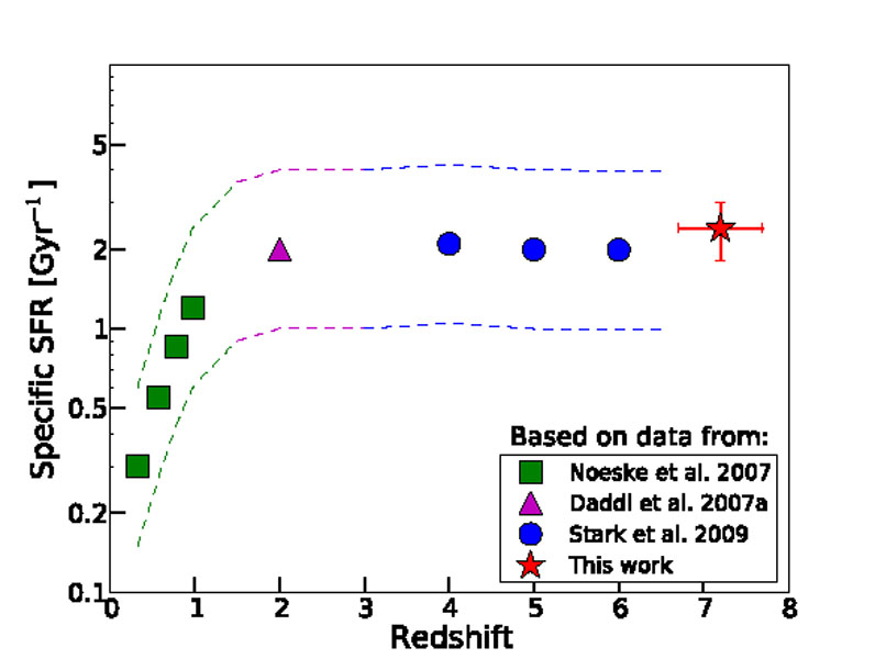 |
Figure 17. Average < sSFR > determined at z ∼ 7 by González et al. (2010) for a median stellar mass of 5 × 10⁹ M⊙ compared to the average values determined by other authors at lower redshifts, but comparable stellar masses (Noeske et al. 2007; Daddi et al. 2007; Stark et al. 2009). This plot implies that < sSFR > stays remarkably constant, at ≃ 2 Gyr-1 over the redshift range 2 < z < 7, suggesting that the star-formation–mass relation does not evolve strongly during the first ≃ 3 billion years of galaxy evolution (courtesy V. González). |
Our current best estimate of the evolving stellar mass function of LBGs at z = 4, 5, 6 & 7 is shown in Fig. 18. This summarizes the work of González et al. (2011), who used the WFC3/IR ERS data in tandem with the GOODS-South IRAC and HST ACS data to establish a mass to luminosity relation Mstar ∝ L15001.7 at z ∼ 4, and then applied this to convert the UV LFs of Bouwens et al. (2007, 2010) into stellar mass functions at z ≃ 4, 5, 6 & 7.
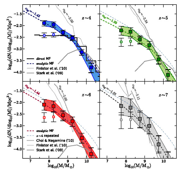 |
Figure 18. The stellar mass functions of LBGs at z ∼ 4, 5, 6, and 7 as produced by González et al. (2011) by applying the Mstar - L1500 distribution found for z ∼ 4 B-dropouts (within the WFC3/IR ERS field) to the UV LFs of Bouwens et al. (2007, 2010) at z ∼ 4-7. For masses Mstar > 109.5 M⊙, the z < 7 mass functions are in reasonable agreement with the earlier determinations by Stark et al. (2009) and McLure et al. (2009). The thick dashed curve in each panel represents the analytic mass functions derived from an idealized Mstar - L1500 relation which, given the adopted form of Mstar ∝ L15001.7, inevitably display somewhat flatter low-mass slopes αmass ≃ -1.4 to -1.6, than the faint-end slopes in the LBG UV LFs (α = -1.7 to-2.0; see section 4.1). The z ≃ 4 analytical mass function is repeated in the other panels for comparison (thin dashed curve). The dotted and thin solid lines show the simulated mass functions from Choi & Nagamine (2010) and Finlator et al. (2011) (courtesy V. González). |
This plot also usefully illustrates both the level of agreement and current tension with current theoretical models, several of which predict extremely steep faint-end mass-function slopes, αmass ≃ -2 to -3 (e.g. Choi & Nagamine 2010; Finlator et al. 2011). The observationally-inferred mass-functions in Fig. 17 appear to display significantly flatter low-mass slopes than this, with αmass ≃ -1.4 to -1.6. However, it must be emphasized that Fig. 18 is based on the assumption that all galaxies at these redshifts follow the same mass-to-light relation as inferred at z ≃ 4 (and even this relation includes many objects without individual IRAC detections, and once again involves the simplifying assumption of constant star-formation rate). Thus the fact that the low-mass end of the mass function has a flatter slope than the faint-end slope of the UV LF is a simple consequence of applying Mstar ∝ L15001.7. In detail this is clearly wrong, but the question is how wrong?
This issue has recently been explored by McLure et al. (2011) who, for 21 galaxies at z > 6.5 which do have IRAC detections, explored the extent to which Mstar for individual galaxies changes if the assumption of a universal Mstar - L1500 relation is relaxed, and the full parameter space of age, star-formation history, dust-extinction and metallicity is explored in search of the best model fit. The results of this analysis are shown in Fig. 19. For individual objects, Mstar can vary considerably depending on the adopted model, and it appears that stellar mass can span a factor of up to ≃ 50 at a given UV luminosity. However, for most objects it is found that the size of the mass uncertainty is generally limited to typically a factor of ≃ 2-3, partly by the lack of available cosmological time (see also Labbé et al. 2010b); this is one (the only?) benefit of working at z > 5, namely that the impact on Mstar of a plausible range of star-formation histories is damped somewhat by the fact that less than 1 billion years is available. Another interesting outcome of this analysis is that, despite the increase in scatter in Mstar, the average value was indeed still found to be consistent with < sSFR > ≃ 2-3 Gyr-1, and McLure et al. (2011) also confirmed that the mass-luminosity relation at z ≃ 7 is at least consistent with the z ≃ 4 relation adopted by González et al. (2011).
 |
Figure 19. Star-formation rate versus stellar mass for the twenty-one objects in the final robust z > 6.5 LBG sample of McLure et al. (2011) with IRAC detections at either 3.6 μm or 3.6+4.5 μm. In the left-hand panel the star-formation rates and stellar masses have been measured from the best-fitting SED template drawn from a wide range of star-formation histories, metallicities and reddening. In the right-hand panel the star-formation rates and stellar masses have been estimated from the best-fitting constant star-formation model. The 1σ errors on both parameters have been calculated by determining the Δχ2 = 1 interval, after marginalising over all other free parameters. The solid line in both panels is the SFR-Mstar relation derived by Daddi et al. (2007) for star-forming galaxies at z ≃ 2 and corresponds to a sSFR of ≃ 2.5 Gyr-1. The dotted lines illustrate how the SFR-Mstar relation for a galaxy with a constant star-formation rate and zero reddening varies as a function of stellar population age, as marked in the right-hand panel (courtesy R. McLure). |
From these plots it can be seen that the typical stellar mass of an L* LBG detected at z ≃ 7 in the current deep WFC3/IR imaging surveys is Mstar ≃ 2 × 10⁹ M⊙, and the faintest LBGs uncovered at these redshifts have masses as low as Mstar ≃ 1 × 10⁸ M⊙ (see also Finkelstein et al. 2010). This is impressive, as is the effort to establish the typical masses of faint LAEs from stacking of the available (somewhat shallower) IRAC imaging over the wider-area narrow-band Subaru surveys. This work indicates even lower typical stellar masses for LAEs selected at z ≃ 5.7 and z ≃ 6.6, with Mstar ≃ 1 - 10 × 107 M⊙ (Ono et al. 2010).
This is not to say that a few significantly more massive LAEs have not been uncovered. For example, Ouchi et al. (2009a) discovered "Himiko", a giant LAE at z = 6.595, whose relatively straightforward IRAC detection implies a stellar mass in the range Mstar = 0.9 - 5 × 10¹¹ M⊙. The example of Himiko shows that reasonably massive galaxies can be uncovered at z ≃ 7 given sufficiently large survey areas (in this case the parent z ≃ 6.6 narrow-band survey covered ≃ 1 deg2, sampling a comoving volume of ≃ 800,000 Mpc3; Ouchi et al. 2010). Such discoveries are "expected", and are entirely consistent with the mass functions shown in Fig. 18. However, one should obviously be sceptical about claims of enormously massive (e.g. Mstar > 5 × 10¹¹ M⊙) galaxies at z > 5, especially at very high redshift and/or if discovered from very small surveys (e.g. Mobasher et al. 2005). In fact, Dunlop et al. (2007) found no convincing evidence of any galaxies with Mstar > 3 × 10¹¹ M⊙ at z > 4 in 125 arcmin2 of the GOODS-South field, a result which is again consistent with the high-mass end of the mass functions shown in Fig. 18.
Given the growing evidence that < sSFR > is approximately constant at early times, it is tempting to conclude that the star-formation rates of high-redshift galaxies are exponentially increasing with time (rather than staying constant or exponentially decaying, as generally previously assumed – e.g. Eyles et al. 2007; Stark et al. 2009). While the analysis of McLure et al. (2011) indicates that it may be a mistake to assume all individual galaxies grow in this self-similar manner, and simple exponential growth is not really supported by the González et al. (2011) mass-luminosity relationship, on average something at least close to this scenario does indeed appear to be broadly consistent with much of the available data from z ≃ 8 down to z ≃ 3 (González et al. 2010; Papovich et al. 2011). Interestingly, the latest results from hydrodynamical simulations strongly predict that the star-formation rates of high-redshift galaxies should be increasing approximately exponentially (e.g. Finlator et al. 2011). However, the same simulations make the generic prediction that < sSFR > should continue to rise with increasing redshift beyond z ≃ 2, with < sSFR > ∝ (1 + z)2.5, tracking the halo mass accretion rate (e.g. Dekel et al. 2009). Thus, if the improving data continue to support an unevolving value for < sSFR > at high redshift, it will likely be necessary to invoke an additional feedback mechanism to supress star-formation in the theoretical models at high redshift.
It is probably premature to attempt to say anything much more detailed about the evolution of the stellar populations in LBGs and LAEs at z ≃ 5-8. Without high-quality spectroscopy, the determination of detailed star-formation histories is inevitably confused by the complications and degeneracies arising from uncertain dust extinction, nebular emission, and metallicity, issues which are discussed a bit further below in the context of UV slopes and ionizing photon escape fractions. Certainly, the best-fitting star-formation histories for z ≃ 7 LBGs deduced by McLure et al. (2011) range from 10 Myr-old "Bursts" to models involving constant star-formation over 700 Myr, and for each individual object a wide range of alternative star-formation histories is generally statistically permitted by the broad-band photometric data and the uncertainty in metallicity. Meanwhile, for LAEs, ages as young as 1-3 Myr have been inferred for the fainter, bluer objects (e.g. Ono et al. 2010).
Of course, as argued by Stark et al. (2009), in reality the star formation in these young galaxies may be highly intermittent or episodic. Interestingly, it is possible to try to estimate the "duty cycles" of LBGs and LAEs by reconciling their clustering properties with their number density. As discussed by Ouchi et al. (2010), the clustering of LAEs at z ≃ 6.6 can be used to infer a typical halo mass of Mhalo ≃ 108 - 109 M⊙, and then comparison of the predicted number-density of such halos with the observed number density of LAEs implies that these galaxies/halos are observable as LAEs for 1-10% of the time. These estimates are clearly still highly uncertain, not least because the clustering properties of LAEs and LBGs are still not very well determined (see section 5.5 below), and indeed, based on the luminosity function comparison discussed above, it could be argued that the duty cycles of LAE and LBG activity must be virtually the same at z ≃ 6 - 7. Nevertheless, such calculations have the potential to provide genuinely useful constraints on duty cycles, as future surveys for z ≃ 5-8 LAEs and LBGs increase in both area and depth.
The first galaxies, by definition, are expected to contain very young stellar populations of very low metallicity. However, the possibility of detecting unambiguous observable signatures of such primordial stellar populations with current or indeed planned future instrumentation is currently a matter of considerable debate.
For example, one long-sought distinctive spectral signature of the first generation of galaxies is relatively strong HeII emission at λrest = 1640 Å (e.g. Shapley et al. 2003; Nagao et al. 2008; di Serego Alighieri et al. 2008). However, near-infrared spectroscopy of the sensitivity required to detect this line at z > 7 will certainly not be available until the JWST, and even then some theoretical predictions indicate that it is unlikely to be found in detectable objects (Salvaterra, Ferrara & Dayal 2011, but see also Pawlik, Milosavljevic & Bromm 2011).
By necessity, therefore, recent attention has focussed on whether the broad-band near-infrared photometry which has now been successfully used to discover galaxies at z ≃ 6.5 - 8.5 can actually be used to establish the rest-frame continuum slopes of the highest redshift galaxies. Specifically, very young, metal-poor stellar populations are arguably expected to result in substantially bluer continuum slopes around λrest ≃ 1500 Å than have been detected to date in galaxies discovered at any lower redshift z < 6.5 (e.g. Steidel et al. 1999; Meurer et al. 1999; Adelberger & Steidel 2000; Ouchi et al. 2004; Stanway et al. 2005; Bouwens et al. 2006; Hathi et al. 2008; Bouwens et al. 2009b; Erb et al. 2010).
It has become the normal convention to parameterise the ultra-violet continuum slopes of galaxies in terms of a power-law index, β, where fλ ∝ λβ (e.g. Meurer et al. 1999; thus, β = -2 corresponds to a source which has a flat spectrum in terms of fν, and hence has zero colour in the AB magnitude system). As discussed by several authors, while the bluest galaxies observed at z ≃ 3 - 4 have β ≃ -2, values as low (i.e. blue) as β = -3 can in principle be produced by a young, low-metallicity stellar population (e.g. Bouwens et al. 2010b; Schaerer 2002). However, as illustrated in Fig. 20, for this idealized prediction to actually be realized in practice, several conditions have to be satisfied simultaneously, namely i) the stellar population has to be very young (e.g. t < 30 Myr for metallicity Z ≃ 10-3 Z⊙, or t < 3 Myr for Z ≃ 10-2 Z⊙), ii) the starlight must obviously be completely free from any significant dust extinction, and iii) the starlight must also not be significantly contaminated by (redder) nebular continuum (a condition which has important implications for UV photon escape fraction, and hence reionization – see, for example, Robertson et al. 2010).
 |
Figure 20. Theoretical predictions of galaxy UV-slope β showing the values that are expected for stellar populations of different age and metallicity, and the reason for the interest generated by intial claims that faint galaxies at z ≃ 7 display < β > ≃ -3 (Bouwens et al. 2010a). The left-hand panel shows the predicted evolution of β for instantaneous starbursts of differing metallicity, with and without predicted nebular continuum (Schaerer 2003). The right-hand panel shows equivalent information for the (arguably more realistic) case of continuous star-formation. More recent measurements of < β > have failed to find evidence for values < β > < -2.5 at z ≃ 7, and have converged on < β > = -2.1 ± 0.1 for brighter (L*) galaxies at z ≃ 7. These plots show that while extreme values of < β > < -2.8 would imply both very low metallicity, and a high UV-photon escape fraction, the interpretation of the more moderate values actually observed (i.e. < β > = -2.0 → -2.5), is much less straightforward. |
For this reason, the report by Bouwens et al. (2010a) (supported to some extent by Finkelstein et al. 2010) that the faintest galaxies detected at z > 6.5 apparently display an average value of < β > = -3.0 ± 0.2 was both exciting and arguably surprising, and was immediately subjected to detailed theoretical interpretation (e.g. Taniguchi et al. 2010).
However, a series of further observational studies of UV slopes over the last year have failed to confirm this result, revealing that the original measurement was biased towards excessively blue slopes in a subtle but significant way (e.g. Dunlop et al. 2012; Wilkins et al. 2011b; Finkelstein et al. 2012; Bouwens et al. 2012). It now seems likely that, for the faintest galaxies uncovered so far at z ≃ 7, the average UV power-law index lies somewhere in the range < β > = -2.5 → - 2.0. As can be seen from Fig. 20, the correct interpretation of such slopes is unclear, as they can be produced by different mixes of age, metallicity, and nebular contributions; it is only in the extreme case of < β > ≃ -3.0 that the interpretation in favour of exotic stellar populations and large escape fractions becomes relatively clean.
Although these more moderate UV slopes are arguably in better accord with theoretical expectations (e.g. Dayal & Ferrara 2012) it may still be the case that some individual galaxies at z ≃ 7 with β = -3 have already been discovered among the faint LBG or LAE samples (e.g. Ono et al. 2010). Unfortunately, however, this is impossible to check with current data because β is such a sensitive function of observed colour. At z ≃ 7, the estimate of β for an HST-selected LBG has currently to be based on a single colour, with
 |
(7) |
Thus, a perfectly "reasonable" photometric uncertainty of ≃ 15% in J125 and H160 translates to a ≃ 20% uncertainty in colour and hence to an 1-σ uncertainty of ± 0.9 in β. Better photometric accuracy, ideally combined with additional near-infrared wavebands to allow improved power-law or SED fitting (as is already possible at lower redshifts; Finkelstein et al. 2012; Castellano et al. 2012) is required to enable a proper investigation of the UV slopes of the faintest galaxies at z ≃ 7 - 8.
In contrast to this confusion at the faintest luminosities, there does at least seem to be general agreement that the brighter galaxies found at z ≃ 7 (with M1500 ≃ -21) have < β > = -2.1 ± 0.1. This is basically as expected for a few hundred Myr-old star-forming galaxy, with solar metallicity and virtually no dust extinction, although other interpretations are possible (see Fig. 20). Certainly, for galaxies at these brighter luminosities, any evolution in < β > with redshift has generally been interpreted as arising predominantly from a change in the level of dust obscuration, as already discussed above in the context of Lyman-α emission. In particular, Bouwens et al. (2009b) have reported that the average value of β exhibited by brighter LBGs declines from < β > ≃ -1.5 at z ≃ 4 to < β > ≃ -2 at z ≃ 6, and have interpreted this as reflecting a progressive reduction in average extinction with increasing redshift. This is an important result, because it leads to the conclusion that the correction to be applied to observed UV luminosity density to account for dust-obscured star-formation steadily decreases with increasing redshift. This has obvious implications for the inferred history of cosmic star-formation density as discussed further below in section 6.1. However, the precise redshift dependence of average extinction, and indeed whether there exists a clear relationship between UV luminosity and spectral slope at high redshift is still the subject of some controversy (Dunlop et al. 2012; Bouwens et al. 2012; Finkelstein et al. 2012; Castellano et al. 2012).
5.4. Galaxy sizes and morphologies
Only the most basic information is known about the morphologies of LBGs and LAEs at z > 5, for the simple reason that the objects are faint, and are thus generally detected at only modest signal:noise ratios. Oesch et al. (2010b) investigated the first WFC3/IR imaging of LBGs at z ≃ 7 - 8, and were able to show that almost all of these galaxies are marginally resolved, with an average intrinsic size of ≃ 0.7 ± 0.3 kpc. Thus, known extreme-redshift LBGs are clearly very compact (certainly too compact to be resolved with typical ground-based imaging), and the detection of extended features is, to date, rare. Comparison with the sizes of LBGs at lower redshift implies that average size decreases gently from z ≃ 4 to z ≃ 7, following approximately a relationship of the form (1 + z)-1 (Fig. 21). A slow decrease in average size at a fixed luminosity with increasing look-back time is anticipated from semi-analytic models of galaxy formation (e.g. Mo et al. 1998, 1999; Somerville et al. 2008; Firmani et al. 2009), and is consistent with earlier observations of lower-redshift LBGs (e.g. Ferguson et al. 2004; Bouwens et al. 2004b) and disc galaxies (e.g. Buitrago et al. 2008). However, it is still unclear whether the apparently observed relationship at high redshift is, at least in part, a consequence of the fact that galaxy detection with HST is biased towards objects which have high surface brightness (e.g. Grazian et al. 2011). Oesch et al. (2010b) claim that this is not a significant problem, but HST imaging covering a greater dynamic range, and providing larger samples for stacking, should certainly help to clarify this issue in the near future.
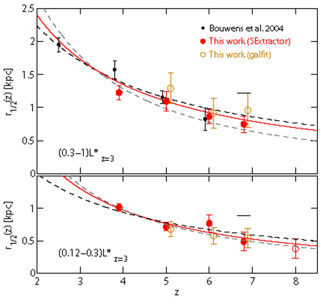 |
Figure 21. The observed evolution of the mean size of Lyman-break galaxies reported by Oesch et al. (2010b), over the redshift range z ∼ 2-8 in two different luminosity ranges (0.3-1)Lz=3* (top) and (0.12-0.3)Lz=3* (bottom) (where Lz=3* is the characteristic luminosity of a LBG at z ≃ 3). Different symbol styles correspond to different ways of analysing the data to extract size estimates. The dashed lines indicate the scaling expected for a fixed dark matter halo mass (∝ (1 + z)-1 ≡ ∝ H(z)-2/3; black) or at fixed halo circular velocity (∝ (1 + z)-3/2 ∝ H(z)-1; gray). The solid red lines indicate the best fit to the observed evolution, which is described as proportional to (1 + z)-m, with m = 1.12 ± 0.17 for the brighter luminosity bin, and m = 1.32 ± 0.52 at fainter luminosities (but both are formally identical, and consistent with m ≃ 1). The extent to which this apparent relationship is influenced by the surface-brightness bias inherent in deep HST imaging is still a matter of some debate (courtesy P. Oesch) |
At somewhat lower redshifts, Taniguchi et al. (2009) used the HST ACS single-orbit I814 imaging in the COSMOS field to attempt to investigate the morphologies of 85 LAEs at z ≃ 5.7, selected via Subaru narrow-band imaging. The results of this study are somewhat inconclusive, with only 47 LAEs being detected, and approximately half of these being apparently unresolved. Nevertheless, the result is a typical half-light radius of ≃ 0.8 kpc, clearly not inconsistent with that displayed by LBGs at comparable redshifts. Taniguchi et al. (2009) also report that fits to the light profile of their stacked images favour a Sérsic index n ∼ 0.7, more consistent with disc-like or irregular galaxies than with a de Vaucouleurs spheroid.
A measurement of the clustering of high-redshift galaxies is of interest primarily for estimating the characteristic mass of the dark matter halos in which they reside. If this can be established with meaningful accuracy, then a comparison of the observed galaxy number density with that of the relevant halos (as predicted within the concordance Λ-CDM cosmological model) can yield an estimate of the halo occupation fraction, or, equivalently, the duty cycle of a given class of high-redshift galaxy.
The measurement of galaxy clustering at z > 5 is still in its infancy, due primarily to the small sample sizes delivered by current facilities. To date it has been most profitably pursued using the samples of several hundred LAEs selected over degree-scale fields via the narrow-band Subaru imaging targetted at z ≃ 5.7 (Ouchi et al. 2005) and z ≃ 6.6 (Ouchi et al. 2010). Fig. 22 shows the distribution on the sky of the ≃ 200 LAEs at z ≃ 6.6 uncovered in the SXDS field by Ouchi et al. (2010).
To quantify the significance and strength of any clustering present in such images, the standard technique is to calculate the Angular Correlation Function, ω(θ), which represents the excess (or deficit) of objects at a given angular radius from a galaxy relative to that expected from a purely random distribution of galaxies with the observed number counts. This is usually calculated following the prescription of Landy & Szalay (1993), which gives
 |
(8) |
where DD(θ), DR(θ), and RR(θ) are the numbers of galaxy-galaxy, galaxy-random, and random-random pairs normalized by the total number of pairs in each of the three samples.
Considerable care and simulation work is required to calculate ωobs(θ) especially when, as shown by the grey regions in Fig. 22, several areas of the image have to be masked out due to bright stars or image artefacts. As described in detail by Ouchi et al. (2005, 2010), ωobs(θ) is converted to a best estimate of ω(θ), then used to derive a clustering amplitude Aω assuming a power-law correlation function ω(θ) = Aωθ-β, in which β has generally to be fixed rather than fitted given the limited sample size (usually β = 0.8 is adopted on the basis of clustering analyses at lower redshift). Finally Aω is coverted into a physical correlation length r0 using knowledge of the redshift distribution (which is relatively straightforward to establish for narrow-band selected LAEs).
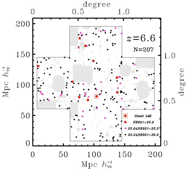 |
Figure 22. The distribution on the sky of the 207 LAEs at z = 6.565 ± 0.054 detected by Ouchi et al. (2010) via narrow-band imaging with Subaru in the SXDS field. Red squares, magenta diamonds, and black circles indicate the positions of bright (NB921 < 25.0), medium-bright (25.0 ≤ NB921 ≤ 25.5), and faint (25.5 ≤ NB921 ≤ 26.0) LAEs, respectively. The red square surrounded by a red open square indicates the giant LAE, Himiko, at z = 6.595 reported by Ouchi et al. (2009a), and already briefly discussed in section 5.1 (courtesy M. Ouchi). |
The result of these studies is that significant clustering has now been detected in the LAE population at z > 5, and that the best estimate of the correlation length for LAEs at z ≃ 5-7 is r0 = 3 - 7 Mpc (for H0 = 70 km s-1 Mpc-1). This in turn can be used to infer an average mass for the dark-matter halos hosting these LAEs of 1010 - 1011 M⊙. A similar analysis for LBGs at 5 < z < 6 has been performed by McLure et al. (2009), who report a correlation length of r0 = 8-1.5+2 Mpc (for H0 = 70 km s-1 Mpc-1) and a resulting characteristic dark-matter halo mass of 1011.5 - 1012 M⊙. This significantly larger halo mass for the LBGs is not unexpected, given that they are considerably rarer, more massive objects (than typical narrow-band selected LAEs), having been selected from a substantially larger cosmological volume, down to much brighter continuum flux limits. These results are consistent with those derived by Overzier et al. (2006) for LBGs at a mean redshift of z ≃ 5.9. Interestingly, the z > 5 LBGs studied by McLure et al. (2009) are bright enough to allow a reasonable estimate of average stellar mass, log10(M / M⊙) = 10.0-0.4+0.2, which is consistent with the results of the clustering analysis for plausible values of the ratio of stellar to dark matter.
Unfortunately the large uncertainty in current estimates of characteristic halo mass, combined with the steepness of the halo mass function, means that such clustering measurements cannot yet be used to yield meaningfully-accurate duty cycles for LAEs and LBGs (e.g. Ouchi et al. (2010) report an inferred duty cycle of ≃ 1% for z ≃ 6.6 LAEs, but acknowledge this is extremely uncertain). Nonetheless, these pioneering studies provide hope for meaningful measurements with the much larger LAE and LBG samples anticipated from Hyper-Suprime Cam on Subaru (Takada 2010) and from the EUCLID Deep survey over the next decade (Laurejis et al. 2011).
As discussed in section 6.2, such future large-scale surveys also have the potential to search for one of the long anticipated signatures of reionization, namely an enhancement in the clustering of LAEs relative to LBGs due to patchy reionization. At present, Ouchi et al. (2010) report no evidence for such a clustering amplitude boost at z ≃ 6.6.