


4.1. Model selection versus parameter estimation
Estimation of cosmological parameters, as described in the previous section, assumes that we have a particular model in mind to explain the data. More commonly, however, there tends to be competing models available to describe the data, invoking parametrizations of different physical effects. Each model corresponds to a different choice of variable parameters, accompanied by a prior distribution for those parameters. Indeed, the most interesting questions in cosmology tend to be those about models, because those are the qualitative questions. Is the Universe spatially flat or not? Does the dark energy density evolve? Do gravitational waves contribute to CMB anisotropies? We therefore need techniques not just for estimating parameters within a model, but also for using data to discriminate between models. Bayesian tools are particularly appropriate for such a task, though I also describe some non-Bayesian alternatives at the end of this section. A comprehensive review of Bayesian model selection as applied to cosmology was recently given by Trotta [26].
An important implication of model-level Bayesian analysis is that there is a clear distinction between a model where a quantity is fixed to a definite value, versus a more general model where that parameter is allowed to vary but happens to take on that special value. A cosmological example is the dark energy equation of state, w, which the cosmological constant model predicts (in good agreement with current observations) to be precisely −1, and which other models such as quintessence leave as a free parameter to be fit from data. Even if it is the cosmological constant which is the true underlying model, a model in which the equation of state can vary will be able to fit any conceivable data just as well as the cosmological constant model (assuming of course that its range of variation includes w = −1). What distinguishes the models is predictiveness.
As an example, consider a magician inviting you to “pick a card, any card”. Since you don't know any better, your ‘model' tells you that are equally likely to pick any card. The one you actually do pick is not particularly surprising, in the sense that whatever it was, it was compatible with your model. The magician, however, has a much more predictive model; by whatever means, they know that you will end up picking the queen of clubs. Both models are equally capable of explaining the observed card, but the magician's much more predictive model lets them earn a living from it. Note in this example, any surprise that you might feel comes not from the card itself, but from the magician's ability to predict it. Likewise, a scientist might find themselves surprised, or dismayed, as incoming data continue to lie precisely where some rival's model said they would.
Model selection/comparison is achieved by choosing a ranking statistic which can be computed for each model, allowing them to be placed in rank order. Within the Bayesian context, where everything is governed by probabilities, the natural choice is the model probability, which has the advantage of having a straightforward interpretation.
The extension of the Bayesian methodology to the level of models is both unique and straightforward, and exploits the normalizing factor P(D) in equation (2) which is irrelevant to and commonly ignored in parameter estimation.
We now assume that there are several models on the table, each with their own probability P(Mi) and explicitly acknowledge that our probabilities are conditional not just on the data but on our assumed model M, writing
 |
(3) |
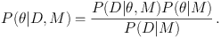
This is just the previous equation with a condition on M written in each term. The denominator, the probability of the data given the model, is by definition the model likelihood, also known as the Bayesian evidence. Note that, unlike the other terms in this equation, it does not depend on specific values for the parameters θ of the model.
The evidence is key because it appears in yet another rewriting of Bayes theorem, this time as
 |
(4) |
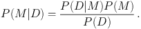
The left-hand side is the posterior model probability (i.e. the probability of the model given the data), which is just what we want for model selection. To determine it, we need to compute the Bayesian evidence P(D|M), and we need to specify the prior model probability P(M). It is a common convention to take the prior model probabilities to be equal (the model equivalent of a flat parameter prior), but this is by no means essential.
To obtain an expression for the evidence, consider Eq. (3) integrated over all θ. Presuming we have been careful to keep our probabilities normalized, the left-hand side integrates to unity, while the evidence on the denominator is independent of θ and comes out of the integral. Hence
 |
(5) |
or, more colloquially,
 |
(6) |
In words, the evidence E is the average likelihood of the parameters averaged over the parameter prior. For the distribution of parameter values you thought reasonable before the data came along, it is the average value of the likelihood.
The Bayesian evidence rewards model predictiveness. For a model to be predictive, observational quantities derived from it should not depend very strongly on the model parameters. That being the case, if it fits the actual data well for a particular choice of parameters, it can be expected to fit fairly well across a significant fraction of its prior parameter range, leading to a high average likelihood. An unpredictive model, by contrast, might fit the actual data well in some part of its parameter space, but because other regions of parameter space make very different predictions it will fit poorly there, pulling the average down. Finally, a model, predictive or otherwise, that cannot fit the data well anywhere in this parameter space will necessarily get a poor evidence.
Often predictiveness is closely related to model simplicity; typically the fewer parameters a model has, the less variety of predictions it can make. Consequently, model selection is often portrayed as tensioning goodness of fit against the number of model parameters, the latter being thought of as an implementation of Ockham's razor. However the connection between predictiveness and simplicity is not always a tight one. Consider for example a situation where the predictions turn out to have negligible dependence on one of the parameters (or a degenerate combination of parameters). This is telling us that our observations lack the sensitivity to tell us anything about that parameter (or parameter combination). The likelihood will be flat in that parameter direction and it will factorize out of the evidence integral, leaving it unchanged. Hence the evidence will not penalize the extra parameter in this case, because it does not change the model predictiveness.
The ratio of the evidences of two models M0 and M1 is known as the Bayes factor [27]:
 |
(7) |
which updates the prior model probability ratio to the posterior one. Some calculational methods determine the Bayes factor of two models directly. Usual convention is to specify the logarithms of the evidence and Bayes factor.
Equation (5) tells us that to get the evidence for a model, we need to integrate the likelihood throughout the parameter space. In principle this is a very standard mathematical problem, but it is made difficult because the integrand is likely to be extremely highly peaked and we do not know in advance where in parameter space the peak might be. Further, the parameter space is multi-dimensional (between about 6 and 10 dimensions would be common in cosmological applications), and as remarked in Section 3 the individual likelihood evaluations of the integrand at a point in parameter space are computationally expensive (a few CPU seconds each), limiting practical calculations to 105 to 106 evaluations. Successful Bayesian model selection algorithms are therefore dependent on efficient algorithms for tackling this type of integral.
Model probabilities are meaningful in themselves and don't require further interpretation, but it is useful to have a scale by which to judge differences in evidence. The usual scale employed is the Jeffreys' scale [7] which, given a difference Δ lnE between the evidences E of two models, reads
| Δ lnE < 1 | Not worth more than a bare mention. |
| 1 < Δ lnE < 2.5 | Significant. |
| 2.5 < Δ lnE < 5 | Strong to very strong. |
| 5 < Δ lnE | Decisive. |
In practice the divisions at 2.5 (corresponding to posterior odds of about 13:1) and 5 (corresponding to posterior odds of about 150:1) are the most useful.
As the main steps in the Jeffreys' scale are 2.5, this sets a target accuracy in an evidence calculation; it should be accurate enough that calculational uncertainties do not move us amongst these different categories. The accuracy should therefore be better than about ± 1. However there is no point in aiming for an accuracy very much better than that, which would not tell us anything further about the relative merits of the models. Hence an accuracy of a few tenths in lnE is usually a good target.
Computing the evidence is more demanding than mapping the dominant part of the posterior, as we now have to be able to accurately integrate the likelihood over the entire parameter space. There are several methods which become exact in the limit of infinite computer time, and are capable of offering the desired accuracy with finite resources. Those used so far in cosmological settings are
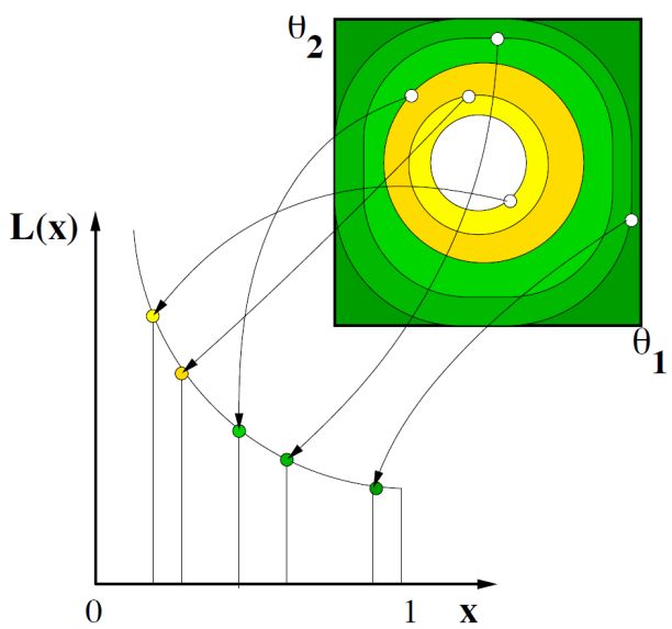 |
Figure 3. A schematic of the nested sampling algorithm. The two-dimensional parameter space is shown at the top right. The points within it are considered to represent contours of constant likelihood, which sit within each other like layers of an onion (there is however no need for them to be simply connected). The volume corresponding to each thin shell of likelihood is computed by the algorithm, allowing the integral for the evidence to be accumulated as shown in the graph. [Figure courtesy David Parkinson.] |
4.3.2. Approximate or restricted methods
In addition to brute force numerical methods to compute the evidence, various approximate or restricted methods exist which may be useful in some circumstances. The most important three, discussed in more detail in Refs. [26, 3], are
 |
(8) |
where  max is the
maximum likelihood achievable by the model, k the number of
parameters, and N the number of datapoints. Models are ranked
according to their BIC values. Despite the name, it has nothing to do
with information theory, but rather was named by analogy to information
theory measures discussed in Section 4.5. It has been
used quite widely in cosmology, but the validity of the approximation
needs careful consideration and full evidence evaluation is to be
preferred whenever possible.
max is the
maximum likelihood achievable by the model, k the number of
parameters, and N the number of datapoints. Models are ranked
according to their BIC values. Despite the name, it has nothing to do
with information theory, but rather was named by analogy to information
theory measures discussed in Section 4.5. It has been
used quite widely in cosmology, but the validity of the approximation
needs careful consideration and full evidence evaluation is to be
preferred whenever possible.
Ultimately, a successful implementation of model selection should result in all models being eliminated except for a single survivor. This model will encode all the physics relevant to our observations, and we can then proceed to estimate the parameters of the surviving model to yield definitive values of quantities of interest, e.g. the baryon density, neutrino masses, etc. Unfortunately, in practice it is quite likely that more than one model might survive in the face of the data, as has always been the case so far in any analysis I've done. Despite that, we might well want to know what the best current knowledge of some of the parameters is.
Fortunately, the Bayesian framework again supplies a unique procedure for extracting parameter constraints in the presence of model uncertainty. One simply combines the probability distribution of the parameters within each individual model, weighted by the model probability. This is very much analogous to quantum mechanics, the superposition of model states being equivalent to a superposition of eigenstates of an observable such as position. The combination is particularly straightforward if one already has a set of samples from the likelihood, such as a Markov chain, for each model; we then just concatenate the chains giving each point a fractional weighting according to the model probability of the chain it came from.
Note that in this superposition, some parameters may have fixed values in some of the models. For example, if we are interested in the dark energy equation of state w, we will no doubt be including a cosmological constant model in which w is fixed to −1. Within this model, the probability distribution is an appropriately normalized delta function, and the combined probability distribution is therefore neither continuous nor differentiable. This can have the interesting consequence that some confidence limits may have zero parameter width. See Ref. [38] for some actual calculations.
4.5. Other approaches to model selection
Within the Bayesian framework, the evidence is the natural model selection statistic. However, other paradigms suggest alternatives. The most prevalent is information theory approaches, where the statistics are known as information criteria. The first and most widespread is the Akaike Information Criterion (AIC), defined by [39]
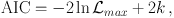 |
(9) |
using the same terminology as equation (8). This sets up a tension between goodness of fit and complexity of the model, with the best model minimizing the AIC. There is also a slightly modified version applicable to small sample sizes, which ought to be used in any case [40]. It is not always clear how big a difference in AIC is required for the worse model to be significantly disfavoured, but a typical guide (actually obtained by attempting a Bayesian-style probabilistic interpretation) is a difference of 6 or more should be taken seriously.
Beyond the AIC, there are a large variety of different information criteria in use. Burham and Anderson [40] give an excellent textbook account of information theory approaches to model selection, and cosmological applications of some of them are discussed in Refs. [3, 41].
Perhaps most worthy of special mention is the Deviance Information Criterion of Spiegelhalter et al. [18], which combines aspects of the Bayesian and information theory approaches. It replaces the k in equation (9) with the Bayesian complexity mentioned towards the end of Section 3.2 (for technical reasons it also replaces the maximum likelihood with the likelihood at the mean parameter values, but this is not so significant). The complexity measures the number of model parameters actually constrained by the data. In doing so it overcomes the main difference between the Bayesian and Information Criterion approaches, which is their handling of parameter degeneracies. The Information Criterion approach penalizes such parameters, but the Bayesian method does not as the integral of the likelihood over the degenerate parameter factors out of the evidence integral. The Bayesian view is that in such cases the more complex model should not be penalized, because the data are simply not good enough to say whether the degenerate parameter is needed or not. As this seems more reasonable, the DIC may be preferable to the AIC.
An alternative model selection approach comes from algorithmic information theory, and has variants known as minimum message length and minimum description length [42]. These interpret the best model as being the one which offers the maximal compression of the data, i.e. that the combination of model plus data can be described in the smallest number of bits. As a concept, this idea remarkably originates with Leibniz in the 17th century.