


5.1. Eternal inflation begets a multiverse
One of the more startling predictions of a variety of inflationary models is the existence of domains outside our observable horizon, where the fundamental constants of nature, and perhaps the effective laws of physics more generally, vary (Guth 1981; Guth and Weinberg 1983; Steinhardt 1983; Vilenkin 1983; Linde 1983, 1986a, 1986b). More specifically: such a `multiverse' arises through eternal inflation, in which once inflation begins, it never ends. 19 Eternal inflation is predominantly studied in two broad settings: (1) false-vacuum eternal inflation and (2) slow-roll eternal inflation.
(1): False-vacuum eternal inflation can occur when the inflaton field ϕ, which is initially trapped in a local minimum of the inflaton potential V(ϕ) (a state that is classically stable but quantum mechanically metastable-i.e., a `false' vacuum), either:
(a) tunnels out of the local minimum to a lower minimum of energy-density, in particular to the `true vacuum', i.e. the true ground state: (as described by Coleman and De Luccia (1980)); or
(b) climbs, thanks to thermal fluctuations, over some barrier in V(ϕ), to the true vacuum.
The result is generically a bubble (i.e. a domain) where the field value inside approaches the value of the field at the true vacuum of the potential. If (i) the rate of tunneling is significantly less than the expansion-rate of the background spacetime, and-or (ii) the temperature is low enough, then the "channels" (a) and-or (b) by which the field might reach the true vacuum are frustrated. That is: inflation never ends, and the background inflating space-time becomes populated with an unbounded number of bubbles. (Cf. Guth and Weinberg (1983); and see Sekino et al. (2010) for a recent discussion of the various topological phases of false-vacuum eternal inflation that can arise in a simplified setting.) 20
(2): In slow-roll eternal inflation, quantum fluctuations of the inflaton field overwhelm the classical evolution of the inflaton in such a way as to prolong the inflationary phase in some regions of space. When this is sufficiently probable, eternal inflation can again ensue; (Vilenkin 1983, Linde 1986a, 1986b; see Guth (2007) for a lucid summary, and Creminelli et al. (2008) for a recent discussion). It is striking that the self-same mechanism that gives rises to subtle features of the CMB (as discussed in Section 4.2.2), can, under appropriate circumstances, give rise to a multiverse.
Though it is not clear how generic the phenomenon of eternal inflation is (Aguirre 2007a; Smeenk 2014), it remains a prediction of a wide class of inflationary models. So in this Section, we turn to difficulties about confirming cosmological theories that postulate a multiverse. Thus we will assume that the multiverse consists of many (possibly an infinite number of) domains, each of whose inhabitants (if any) cannot directly observe, or otherwise causally interact with, other domains; (though we will soon mention a possible exception to this).
There is a growing literature about these difficulties. It ranges from whether there could, after all, be direct experimental evidence for the other universes, to methodological debates about how we can possibly confirm a multiverse theory without ever having such direct evidence.
We focus here on the methodological debates. 21 Thus for us, the main theme will be - not that it is hard to get evidence - but that what evidence we get may be greatly influenced by our location in the multiverse. In the jargon: we must beware of selection effects. So one main, and well-known, theme is about the legitimacy of so-called anthropic explanations. In broad terms, the question is: how satisfactory is it to explain an observed fact by appealing to its absence being incompatible with the existence of an observer?
We of course cannot take on the large literature about selection effects and anthropic explanations: (cf. e.g. Davies (1982); Barrow and Tipler (1988); Earman (1987); Rees (1997); Bostrom (2002); McMullin (1993, 2005, 2007); Mosterín (2005)); Carr (2007); Landsman (2016)). We will simply adopt a scheme for thinking about these issues, which imposes a helpful `divide and rule' strategy on the various (often cross-cutting and confusing!) considerations (Section 5.2). This scheme is not original to us: it combines proposals by others-mainly: Aguirre, Tegmark, Hartle and Srednicki. Then in Section 5.3, we will report results obtained by one of us (Azhar (2014, 2015, 2016)), applying this general scheme to toy models of a multiverse (in particular, models about the proportions of various species of dark matter). The overall effect will be to show that there can be a severe problem of under-determination of theory by data.
In this Section, we will adopt a scheme that combines two proposals due to others:
(i) a proposal distinguishing three different problems one faces in extracting from a multiverse theory, definite predictions about what we should expect to observe: namely, the measure problem, the conditionalization problem, and the typicality problem (Aguirre and Tegmark (2005) and Aguirre (2007b)); (Section 5.2.1);
(ii) a proposal due to Srednicki and Hartle (2007, 2010) to consider the confirmation of a multiverse theory in Bayesian terms (Section 5.2.2).
5.2.1. Distinguishing three problems: measure, conditionalization, and typicality
Our over-arching question is: given some theory of the multiverse, how should we extract predictions about what we should expect to observe in our domain? Aguirre puts the question well:
Imagine that we have a candidate physical theory and set of cosmological boundary conditions (hereafter denoted
) that predicts an ensemble of physically realized systems, each of which is approximately homogeneous in some coordinates and can be characterized by a set of parameters (i.e. the constants appearing in the standard models of particle physics and cosmology; I assume here that the laws of physics themselves retain the same form). Let us denote each such system a "universe" and the ensemble a "multiverse". Given that we can observe only one of these universes, what conclusions can we draw regarding the correctness of
Thus we want to somehow define the probability, assuming
, of a given value,
 say, of a set of
observables. But calculational complexities and selection effects make
this difficult. Aguirre goes on to propose a helpful `divide and rule'
strategy, which systematizes the various considerations one has to
face. In effect, there are three problems, which we now describe.
22
say, of a set of
observables. But calculational complexities and selection effects make
this difficult. Aguirre goes on to propose a helpful `divide and rule'
strategy, which systematizes the various considerations one has to
face. In effect, there are three problems, which we now describe.
22
5.2.1.A: The measure problem: To define a probability
distribution P, we first need to specify the sample space: the
type of object M that are its elements - traditionally called
`outcomes', with sets of them being called `events'. Each observable
will then be a random variable on the sample space, so that for a set
of observables
,
P()
is well-defined. One might take each M to be a domain in the
sense above, so that P() represents the probability of
occurring in a randomly chosen domain: where P may, or may not,
be uniform on the sample space.
23
But it is not clear a priori that domains should be taken as the
outcomes, i.e. the basic alternatives. For suppose, for example, that
says domains in which our
observed values occur are much smaller than domains where they do not
occur. So if we were to split each of these latter domains into domains
with the size of our domain, the probabilities would radically
change. In short, the problem is that there seems no a priori best way
of selecting the basic outcomes.
Besides, this problem is made worse by various infinities that arise in eternal inflation. Mathematically natural measures over reasonable candidates for the outcomes often take infinite values, and so probabilities often become ill-defined; (including when they are taken as ratios of measures). Various regularization schemes have been introduced to address such issues; but the probabilities obtained are not independent of the scheme used. This predicament-the need, for eternally inflating space-times, to specify outcomes and measures, and to regularize the measures so as to unambiguously define probabilities-is known as the measure problem. For a review of recent efforts, cf. Freivogel (2011). (Note that this measure problem is not the same as the problems besetting defining measures over initial states of a cosmological model, as in (3) at the end of Section 1: cf. Carroll (2014: footnote 13).
5.2.1.B: The conditionalization problem: Even if one has a
solution to the measure problem, a second problem arises. It is
expected, that for any reasonable
and any reasonable
solution to the measure problem, the probabilities for what we
will see will be small. For in eternal inflation, generically, much of
the multiverse is likely to not resemble our domain. Should we thus
conclude that all models of eternal inflation are disconfirmed? We might
instead propose that we should restrict attention to domains (or more
generally: regions) of the multiverse, where we can exist. That is, we
should conditionalize: we should excise part of the sample
space and renormalize the probability distribution, and then compare the
resulting distribution with our observations. This process of
conditionalization can be performed in three main ways; (see
Aguirre and Tegmark 2005):
(i) we can perform no conditionalization at all - known as the "bottom-up" approach;
(ii) we can try to characterize our observational situation by selecting observables in our models that we believe are relevant to our existence (and hence for any future observations and experiments that we may make) - known as the "anthropic approach";
(iii) we can try to fix the values of each of the observables in our models, except for the observable we are aiming to predict the value of - known as the "top-down" approach.
As one might expect, there are deep, unresolved issues, both technical and conceptual, for both (ii) and (iii) above. For the anthropic approach, (ii), one faces the difficult question of how precisely to characterize our observational situation, and so which values of which observables we should conditionalize on. In the top-down approach, (iii), it is unclear how we can perform this type of conditionalization in a practical way.
And on both approaches, we expect the observable we aim to predict the value of and the conditionalization scheme to be separated in an appropriate way-but it is not clear how to go about doing this. It is natural to require that the observable being predicted:
(a) is correlated with the conditionalization scheme (otherwise the conditionalization scheme would play no role in the predictive framework), but:
(b) is not perfectly correlated with the conditionalization scheme (otherwise one would be open to the charge of circularity).
So when it is not clear exactly how observables are correlated with the defining features of a conditionalization scheme-as indeed it is not in eternal inflation!-the need to strike a balance between these two requirements amounts to a difficult problem. In short, the problem is: how can we distinguish the observable to be predicted, from the defining features of the conditionalization scheme? (See Garriga and Vilenkin (2008, Section III) who mention such concerns, and Hartle and Hertog (2013).)
5.2.1.C: The typicality problem: Even if one has solved (at least to one's own satisfaction!) both the measure and conditionalization problems, a third problem remains: the typicality problem. Namely: for any appropriately conditionalized probability distribution, how typical should we expect our observational situation to be, amongst the domains/regions, to which the renormalized probability distribution is now restricted? In other words: how much "away from the peak, and under the tails" can our observations be, without our taking them to disconfirm our model? In the next Section, we will be more precise about what we mean by `typicality'; but for now, the intuitive notion will suffice.
Current discussions follow one of two distinct approaches. One approach asserts that we should always assume typicality with respect to an appropriately conditionalized distribution. This means we should assume Vilenkin's "principle of mediocrity", or something akin to it (Gott (1993); Page (1996); Vilenkin (1995); Bostrom (2002); Garriga and Vilenkin (2008)). The other approach asserts that the assumption of typicality is just that-an assumption-and is thus subject to error. So one should allow for a spectrum of possible assumptions about typicality; and in aiming to confirm a model of eternal inflation, one tests the typicality assumption, in conjunction with the measure and conditionalization scheme under investigation. This idea was developed within a Bayesian context most clearly by Srednicki and Hartle (2007, 2010); and it is to a discussion of their scheme that we now turn.
5.2.2. The Srednicki-Hartle proposal: frameworks
Srednicki and Hartle
(2010)
argue that in what they call a "large universe" (i.e. a multiverse), we
test what they dub a framework: that is, a conjunction
of four items: a cosmological (multiverse) model
, a measure, a
conditionalization scheme, and an assumption about typicality. (Agreed,
the model might specify
the measure; but it can hardly be expected to specify the
conditionalization scheme and typicality assumption.)
If such a framework does not correctly predict our observations, we have license to change any one of its conjuncts, 24 and to then compare the distribution derived from the new framework with our observations. One could, in principle, compare frameworks by comparing probabilities for our observations against one another (i.e., by comparing likelihoods); or one can formulate the issue of framework confirmation in a Bayesian setting (as Srednicki and Hartle do).
To be more precise, let us assume that a multiverse model
includes a prescription
for computing a measure, i.e. includes a proposed solution to the
measure problem: this will simplify the notation. So given such a model
, a conditionalization
scheme  , and a typicality
assumption, which for the moment we will refer to abstractly as ξ:
we aim to compute a probability distribution for the value
D0 of some observable. We write this as
P(D0|
,
, ξ). Bayesian
confirmation of frameworks then proceeds by comparing posterior
distributions P,(,
,
ξ|D0), where
, and a typicality
assumption, which for the moment we will refer to abstractly as ξ:
we aim to compute a probability distribution for the value
D0 of some observable. We write this as
P(D0|
,
, ξ). Bayesian
confirmation of frameworks then proceeds by comparing posterior
distributions P,(,
,
ξ|D0), where
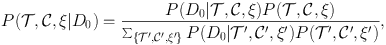 |
(5.1) |
and P(,
, ξ) is a prior over
the framework {,
, ξ}.
How then do we implement typicality assumptions?
Srednicki and Hartle
(2010)
develop a method for doing so by assuming there are a finite number
N of locations where our observational situation
obtains. Assumptions about typicality are made through "xerographic
distributions" ξ, which are probability distributions encoding our
beliefs about at which of these N locations we
exist. So if there are space-time locations xA, with
A = 1,2,...,N, where our observational situation obtains,
the xerographic distribution ξ is a set of N numbers ξ
≡ {ξA}A=1N, such that
∑A=1N ξA = 1. Thus typicality
is naturally thought of as the uniform distribution, i.e.,
ξA = 1 / N. Assumptions about various forms of
atypicality correspond to deviations from the uniform
distribution. Likelihoods P(D0|,
, ξ) in Eq. (2) can
then be computed via: P(D0|
,
, ξ) =
∑A=1N
ξAP(D0[A]
| ,
), where
D0[A] denotes that D0 occurs
at location A. (Admittedly, this equation is somewhat schematic:
see Srednicki and Hartle
(2010:
Appendix B) and
Azhar (2015:
Section II A and III) for more detailed implementations).
In this way, different assumptions about typicality, expressed as different choices of ξ, can be compared against one another for their predictive value. Azhar (2015) undertakes the task of explicitly comparing different assumptions about typicality in simplified multiverse cosmological settings. He shows that for a fixed model, the assumption of typicality i.e. a uniform xerographic distribution (with respect to a particular reference class) achieves the maximum likelihood for the data D0 considered. But typicality does not necessarily lead to the highest likelihoods for our data, if one allows different models to compete against each other.
This conclusion is particularly interesting when for some model, the assumption of typicality is not the most natural assumption. Hartle and Srednicki (2007: Section II) make the point with an amusing parable. If we had a model according to which there were vastly more sentient Jovians than Earthlings, we would surely be wrong, ceteris paribus, to regard the natural corresponding framework as disconfirmed merely by the fact that according to it, we are not typical observers. That is: it is perfectly legitimate for a model to suggest a framework that describes us as untypical. And if we are presented with such a model, we should not demand that we instead accept another model under which typicality is a reasonable assumption. Indeed, demanding this may lead us to choose a framework that is less well confirmed, in Bayesian terms. 25
5.3. Different frameworks, same prediction
As an example of how the scheme described in Section 5.2.2 can lead to further interesting insights, we describe recent work that investigates simplified frameworks in toy models of a multiverse. The results will again illustrate the main theme of this chapter: the under-determination of theory by data. 26
Aguirre and Tegmark (2005) considered a multiverse scenario in which the total number of species of dark matter can vary from one domain to another. They assumed the occurrence of the different species to be probabilistically independent of one another; and then investigated how different conditionalization schemes can change the prediction of the total number of dominant species (where two or more species are called `dominant' when they have comparable densities, each of which is much greater than the other species' density). Azhar (2016) extended this analysis, by considering (i) probabilistically correlated species of dark matter, and (ii) how this prediction varies when one makes various assumptions about our typicality, in the context of various conditionalization schemes. We will thus conclude this Section by outlining one example of this sort of analysis, and highlighting the conclusions about under-determination thus obtained.
In the notation of Section 5.2.1; assume that
is some multiverse model
(with an associated measure), which predicts a total of N
distinct species of dark matter. We assume that from this theory we can
derive a joint probability distribution P(η1,
η2, ..., ηN|) over the densities of
different dark matter species, where the density for species i,
denoted by ηi, is given in terms of a
dimensionless dark matter-to-baryon ratio ηi: =
Ωi / Ωb. We observe the total
density of dark matter ηobs: =
∑i=1N ηi. In fact, according
to results recently released by the Planck collaboration,
ηobs ≈ 5
(Ade et al. 2015).
In Azhar (2016), some simple probability distributions P(η1, η2, ..., ηN|T) are postulated, from which considerations of conditionalization and typicality allow one to extract predictions about the total number of dominant species of dark matter. The conditionalization schemes studied in Azhar (2016) (and indeed in Aguirre and Tegmark 2005) include examples of the "bottom-up", "anthropic", and "top-down" categories discussed in Section 5.2.1. 27 And considerations of typicality are implemented in a straightforward way, by taking typical parameter values to be those that correspond to the peak of the (appropriately conditionalized) probability distribution. 28
Here is one example of the rudiments of this construction. Top-down conditionalization corresponds to analyzing probability distributions P(η1, η2, ..., ηN|T) along the constraint surface defined by our data, i.e., η: = ∑i=1N ηi ≈ 5. The number of species of dark matter that contribute significantly to the total dark matter density, under the assumption of typicality, is then the number of significant components that lie under the peak of this distribution on the constraint surface.
Azhar (2016) shows that different frameworks can lead to precisely the same prediction. In particular, the prediction that dark matter consists of a single dominant component can be achieved through various (mutually exclusive) frameworks. Besides, the case of multiple dominant components does not fare any better. In this sense, any future observation that establishes the total number of dominant species of dark matter will under-determine which framework could have given rise to the observation.
The moral of this analysis is thus that if in more realistic cosmological settings, this under-determination is robust to the choice of which observable we aim to predict the value of (as one would expect), then we must accept that our observations will simply not be able to confirm any single framework for the inflationary multiverse.
19 This process should more accurately be described as future-eternal inflation. Borde, Guth, and Vilenkin (2003) argue that inflation cannot be past-eternal; but see Aguirre (2007a) for a different interpretation of their results. Back.
20 After about 2000, this type of eternal inflation gained renewed interest in light of the idea of a string landscape, in which there exist multiple such metastable vacua (Bousso and Polchinski 2000; Kachru et al. 2003; Susskind 2003; Freivogel et al. 2006). Back.
21 Direct experimental evidence for the other universes could perhaps be obtained from bubble collisions, i.e. from the observational imprints they might leave in our domain (see Aguirre and Johnson (2011) for a review). But such imprints have not yet been found (Feeney et al. 2011). Back.
22 Features of these problems are implemented in actual calculations by, for example, Tegmark (2005) and Aguirre and Tegmark (2005). But a comprehensive treatment, with each of the three components explored in detail, has yet to be carried out. Back.
23 One imagines that the domains are defined as subsets of a single eternally-inflating (classical) space-time: cf. Vanchurin (2015). Back.
24 Philosophers of science will of course recognize this as an example of the Duhem-Quine thesis. Back.
25 Aficionados of the threat of "Boltzmann brains" in discussions of the cosmological aspects of foundations of thermal physics will recognize the logic of the Jovian parable. We cannot here go into details of the analogy, and the debates about Boltzmann brains; (cf. e.g. Albrecht and Sorbo 2004; De Simone et al. 2010). Suffice it to say that the main point is: a model that implies the existence of many such brains may be implausible, or disconfirmed, or have many other defects; but it is not to be rejected, just because it implies that we-happily embodied and enjoying normal lives!-are not typical. In other words: it takes more work to rebut some story that there are zillions of creatures who are very different from me in most respects, but nevertheless feel like me ("share my observations/experiences"), than just the thought `if it were so, how come I am not one of them?'. For the story might also contain a good account of how and why, though I feel like them, I am otherwise so different. Back.
26 This section is based on Azhar (2014, 2016), which both build upon the work of Aguirre and Tegmark (2005). The scheme we use does not explicitly address the measure problem; we simply assume there is some solution, so that probability distributions over observables of interest can indeed be specified. Back.
27 To be more precise: in the bottom-up and top-down cases, the total number N of species is fixed by assumption, and one looks for the total number of dominant species; while in the anthropic case, N is allowed to vary, and one looks for the total number N of equally contributing components. Back.
28 The issue of how this characterization of typicality relates to xerographic distributions is subtle. It should be clear that for a finite number of domains, the assumption of typicality as encoded by a uniform xerographic distribution corresponds to assuming that we (and thus the parameter values we observe) are randomly `selected' from among the domains, and this is typicality as understood in the straightforward way. The corresponding relationship for the case of atypicality is more nuanced. For with non-uniform xerographic distributions, one has the freedom to choose which of the domains receive which precise (xerographic) weight: a feature that is lost when one assumes that atypicality corresponds to an appropriate deviation from the peak of a probability distribution. Back.