


As noted above, the broad emission-line fluxes are observed to vary in response to continuum variations, with a short (usually days to weeks for typical Seyfert 1 galaxies) time delay that is attributable to the light travel time across the BLR, i.e., τlt = R / c. This affords a potentially powerful tool; by closely examining the velocity-resolved response of the broad lines to continuum variations, the kinematics and geometry of the BLR can be determined, or at least highly constrained. Moreover, while the observations have to be done with great attention to quality and homogeneity, they are not otherwise a serious observational challenge since they involve prominent emission lines in the UV/optical spectra of relatively bright AGNs.
The reverberation method as it is currently applied to AGNs rests on some simple assumptions, e.g., [4, 22, 24], which to some extent can be justified ex post facto:
The continuum originates in a single central source. The continuum source in typical Seyfert galaxies (1013 – 1014 cm) is much smaller than the BLR, which reverberation reveals to be ∼ 1016 cm in these objects. Note in particular that it is not necessary to assume that the radiation from the central source is emitted isotropically.
The light travel time across the BLR is the most important time scale. Specifically, we assume that that cloud response time is instantaneous, which is a good assumption given the high densities of the BLR gas. The response time is given by the recombination time scale τrec = (ne αB)-1 ≈ 0.1(1010 cm-3 / ne) hours, where αB is the hydrogen case B recombination coefficient and ne is the particle density. It is also assumed that the BLR structure is stable over the duration of the reverberation experiment, which is typically no longer than several months for Seyfert galaxies, but can be much longer for high-luminosity quasars. For typical low-luminosity reverberation-mapped AGNs (i.e., Seyfert galaxies), τdyn ≈ 3–5 years.
There is a simple, though not necessarily linear, relationship between theobserved continuum and the ionizing continuum. The key element is that the ionizing continuum and observable (either satellite UV or optical) continuum vary in phase. In only two well-studied cases, NGC 7469 and Akn 564, has this assumption been critically tested. In both cases, time lags between the continuum variations at the shortest UV wavelengths and those at the longest optical wavelengths are of order ∼ 1 day. In terms of amplitude of variation, the variations in the UV are generally much stronger, even after taking dilution of the optical continuum into account.
Under these simple assumptions, a simple linearized model to describe the emission-line light curve as a function of line-of-sight (LOS) velocity V can be written as
 |
(3) |
where ΔC(t) and ΔL(t, V) are the differences from the mean continuum and mean LOS velocity-resolved emission-line light curves, respectively, τ is the time delay, and Ψ(τ, V) is the "transfer function" or, more descriptively, the "velocity-delay map." The velocity-delay map is thus the response of an emission line to an instantaneous or δ-function continuum outburst at some time t0, i.e., C(t) = δ(t - t0). The goal of reverberation mapping is to recover the velocity-delay map from the observables, ΔC(t) and ΔL(t, V), and thus infer the structure and geometry of the line-emitting region. This represents a classical inversion problem in physics, and solution by Fourier methods immediately suggests itself. However, solution by Fourier transforms is successful only in the case of large amounts of data and low noise, neither condition which can be easily realized in astronomical observations of faint sources. A less ambitious goal is to determine the "delay map" Ψ(τ) = ∫ Ψ(τ, V) dV by using the integrated emission-line light curve. In practice, unambiguous determination of delay maps has also been illusive. In most cases, we have to settle for an estimate of the mean time scale for response, which we obtain by cross-correlating the continuum and emission-line light curves; the mean delay time, or "lag," is usually a good estimate of the centroid of the delay map.
As noted above, the velocity-delay map represents the response of the BLR to a δ-function outburst, as seen by a distant observer. At the moment the observer detects the outburst, he will also detect the response of the emission-line gas along his line of sight to the continuum source; the total path followed by the ionizing photons that leave the central source and are replaced by emission-line photons when they encounter the BLR gas is the same path followed by the unabsorbed photons that are eventually detected by the observer. There is thus no time delay for the response of gas along the line of sight to the continuum source. For all other points, however, there will be a time delay τ between detection of the continuum outburst and the line response because of the increased path length.
Suppose for simplicity that the BLR clouds are all in a circular Keplerian orbit of radius r around the central black-hole/accretion-disk structure. At any given delay τ we observe the response of all points on a surface of constant delay, or "isodelay surface," which must be a paraboloid of revolution around the line of sight. This is illustrated in Fig. 2 which shows that, compared to the signal from the central source, the signal from anywhere else on the ring is delayed by light-travel time effects.
 |
Figure 2. For illustrative purposes, BLR clouds are supposed to be on circular Keplerian orbits of radius r and the continuum source is a point at the center of the ring. Following a continuum outburst, at any given time the observer far to the left sees the response of clouds along a surface of constant time delay, or isodelay surface. Here we show five isodelay surfaces, each one labeled with the time delay (in units of the shell radius r) we would observe relative to the continuum source. Points along the line of sight to the observer are seen to respond with zero time delay. The farthest point on the shell responds with a time delay 2r / c. |
In the upper panel of Fig. 3, we define a system of polar coordinates measured from our line of sight to the continuum source. For clouds at position (r, θ), we see that the observer detects a time delay
 |
(4) |
Thus, at any time delay τ relative to the detection of the outburst, the distant observer sees the response of all gas clouds that intersect with the isodelay surface defined by (4).
We are now prepared to construct a simple velocity-delay map from first principles. We adopt as a toy model the edge-on (inclination i = 90°) ring system shown in the upper panel of Fig. 3 and consider now how the points on the ring translate from (r, θ) measured in configuration space to (V, τ) measured in velocity-delay space. This is illustrated in the lower panel of Fig. 3, where we have identified two of the emission-line clouds that lie on a particular isodelay surface. These points obviously project to τ = (1 + cos θ) r / c and LOS velocities V = Vorb sin θ, where Vorb is the circular orbit speed. It is thus easy to see that an edge-on ring in configuration space projects to an ellipse in velocity-delay space, with semi-axes Vorb and r / c. It is also trivial to see that decreasing the inclination of the ring from 90° will decrease both axes by a factor of sin i; as i approaches 0, the velocity-delay ellipse contracts towards a single point at V = 0 (since the orbital motion is now in the plane of the sky) and τ = r / c (since all points on the ring are now equidistant from the observer).
 |
Figure 3. The upper diagram shows a ring-like BLR with the observer to the left. The upper diagram shows a ring (or cross-section of a thin shell) that contains line- emitting clouds, as in Fig. 2. An isodelay surface for an arbitrary time is given; the intersection of this surface and the ring shows the clouds that are observed to be responding at this particular time. The dotted line shows the additional light-travel time, relative to light from the continuum source, that signals reprocessed by the cloud into emission-line photons will incur (4). In the lower diagram, we project the ring of clouds onto the LOS velocity/time-delay (V, τ) plane, assuming that the emission-line clouds in the upper diagram are orbiting in a clockwise direction (so that the cloud upper part of the orbit in the upper diagram is blueshifted and is represented on the left side of the lower diagram). |
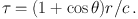
Once we have a velocity-delay map for a ring at arbitrary inclination, it is simple to take the next step to a Keplerian disk, which is essentially a sequence of rings with orbital velocities decreasing like Vorb ∝ r-1/2. Such a sequence of rings is shown in Fig. 4.
 |
Figure 4. Same information as in Fig. 3, except that here, the response is given for a multiple-ring system for clouds in circular Keplerian orbits. Each orbit projects to an ellipse in velocity–delay space. Larger orbits project to larger ranges in time delay (2r / c) and smaller LOS velocities (V ∝ r-1/2). |
Generalization to a disk (a series of rings), a thin shell (a series of rings of fixed r and varying i), or a thick shell (a series of thin shells of varying r) is trivial because of the linear nature of (3). All simple geometries dominated by Keplerian motion will show in the velocity-delay map the same characteristic "taper" with increasing time delay as seen in Fig. 4.
The ultimate goal of reverberation mapping is to recover the velocity-delay map from the observations. Unfortunately, in no case to date has this been possible, though in fairness it must be noted that recovery of a velocity-delay map has not been the principal goal of any experiment that has been carried out as designed; virtually all previous reverberation mapping programs have been designed to measure only the mean response time of emission lines to continuum variations. Even this comparatively modest goal has led to a number of important results, as described below.