4. REVERBERATION RESULTS

4.1. Size of the BLR and Scaling with Luminosity

Emission-line time delays, or lags, have been measured for 35 AGNs, in some cases for multiple emission lines. The highest ionization emission lines are found to respond most rapidly to continuum variations, demonstrating clearly that there is ionization stratification within the BLR. Moreover, the highest ionization lines tend to be broader than the lower ionization lines, and indeed a plot of line width versus time delay shows that the lag τ varies with line width ΔV as τ ∝ ΔV^-2, the virial relationship expected if the dynamics of the BLR is dominated by the gravitational potential of the central source. We show the results for the well-studied case of NGC 5548 in Fig. 5, [26].

Figure 5. Line width, as characterized by the line dispersion (second moment of the profile), versus time delay, as measured by the cross-correlation function centroid τcent, for multiple lines and multiple epochs for NGC 5548. The line measurements are for the variable part of the line only, as isolated by forming a root-mean-square (rms) spectrum from the many spectra obtained in the variability monitoring program. The solid line is the best fit to the data, and the dotted line is a forced fit to slope -1/2, the virial slope; in this particular case, the two lines are indistinguishable. The open circles are measurements of Hβ for 14 different years. The filled circles represent all of the other lines. From [25].

As noted earlier, AGN spectra are remarkably similar over a broad range of luminosity. We might thus infer that, to some low order of approximation, their BLRs have similar physical conditions. Specifically, referring back to (1) and (2), we might conclude that U and n_e are about the same in all AGNs, and from that we could easily reach the conclusion that there should be a very simple relationship between the size of the BLR and the AGN continuum luminosity [16], (since L ∝ Q) of the simple form

(5)

In Fig. 6, we plot the size of the broad Hβ-emitting region as a function of the optical luminosity at 5100 Å for over 30 AGNs, some represented by multiple measurements at different epochs. The observed slope of this correlation, τ(Hβ) ∝ L^{0.6 ± 0.1} is surprisingly consistent with the very naive prediction of (5) over four orders of magnitude in luminosity and time delays ranging from a few days to hundreds of days.

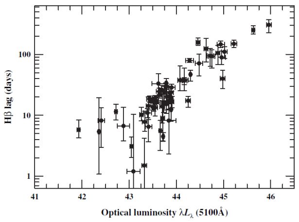Figure 6. Measured time delays for Hβ versus optical luminosity for over 30 reverberation-mapped AGNs, including multiple measurements of some sources. The relationship between BLR size and luminosity can be fitted with r(Hβ) ∝ L0.6 ± 0.1. Based on data from [25].

In the case of the particularly well-observed Seyfert 1 galaxy NGC 5548, the Hβ response time has been measured for 14 individual observing seasons, yielding measured lags ranging from as short as 6 days to as long as 26 days, depending on the mean continuum luminosity. The relationship between Hβ lag and continuum luminosity is shown in Fig. 7. The best-fit slope to this correlation is τ (Hβ) ∝ L^0.9, significantly steeper than the result obtained by comparing different objects. The explanation for this, however, seems to be simple: the shape of the continuum changes as AGNs vary. As the continuum source gets brighter, it also gets harder, i.e., the amplitude of variability is larger at shorter wavelengths. Comparison of the ultraviolet (1350 Å) and optical (5100 Å) continuum fluxes in NGC 5548 shows that L_opt∝ L_UV^0.56, and since the size of the line-emitting region is controlled by the H-ionizing continuum (λ < 912 Å), the UV flux should be a much better measure of the ionizing flux than the optical flux. Thus, we find that

(6)

again, consistent with the naive prediction.

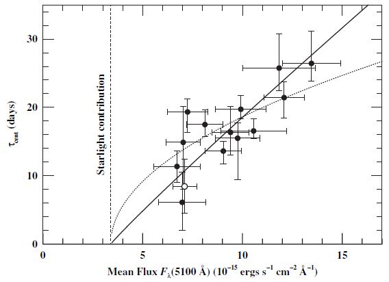Figure 7. Measured time delays for Hβ in NGC 5548 versus optical continuum flux for 14 independent experiments. The vertical line shows the constant stellar contribution to the measured continuum flux. The best-fit slope to this relationship is shown as a solid line τ(Hβ) ∝ Fλ0.9 and the dotted line shows the naive prediction τ(Hβ) ∝ Fλ1/2. From [27].

At least a partial answer is provided by considering the result shown in Fig. 7. What is obvious from this diagram is that the Hβ-emitting gas of the BLR is not changing its location from year to year as the continuum changes; it is obviously not moving fast enough to do this. What we are forced to conclude is that gas is everywhere in the line-emitting region (in this case, at least between ∼ 6 and ∼ 26 light days of the central source) and that what is actually changing with time, or more properly with luminosity, is the distance from the continuum source at which the physical conditions are optimal for emission in the Hβ line. This is often referred to as the "locally optimally-emitting cloud (LOC)" model, e.g., [3]. The basic idea is that line-emitting clouds of gas of various density are distributed throughout the nuclear region. Emission in a particular line comes predominantly from clouds with optimal conditions for that line, and this location can vary as the continuum flux changes. An example of a grid of emission line strengths in an LOC photoionization equilibrium model is shown in Fig. 8.

Figure 8. Contours of constant equivalent width for a grid of photoionization equilibrium models, as a function of input ionizing flux (Φ(H) = Qion / 4 π r2) and particle density n(H) for strong emission lines in AGN spectra. Dotted contours are separated by 0.2 dex and solid contours by 1 dex. The solid star is a reference point to "standard BLR parameters," i.e., the best single-zone model. The triangle shows the location of the peak equivalent width for each line. From [17].

4.2. Reverberation and AGN Black Hole Masses

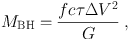
As shown in Fig. 5, for AGNs with multiple reverberation measurements, there is virial relationship between line width and lag. This is strong evidence that the broad lines can be used to measure the mass of the central black hole via the virial theorem,

(7)

where f is a factor of order unity that depends on the unknown geometry and kinematics of the BLR. That these virial masses are valid at some level is demonstrated by the fact that a plot of the reverberation-based masses versus the stellar bulge velocity dispersion σ_∗ is consistent with the same M_BH - σ_∗ relationship seen in quiescent galaxies based on masses measured primarily by stellar or gas dynamics, e.g., [12, 13]. Indeed, a mean value for the scaling factor f in (7) can be obtained by scaling the AGN M_BH - σ_∗ relationship to that for quiescent galaxies. Unfortunately, however, most dynamical models of the BLR give similar values of f, so this affords no useful constraint on the BLR structure and kinematics.

Figure 9 shows the relationship between black hole mass and luminosity for the 35 reverberation-mapped AGNs. All of the AGNs are sub-Eddington, contrary to some earlier estimates, and based on an admittedly nominal bolometric correction, the accretion rates are typically about 10% of the Eddington rate, but with considerable scatter about this value. The scatter in this mass-luminosity relationship is apparently real; the NLS1s occupy the right-hand edge of the envelope, as expected, and the one reverberation-mapped AGN with very broad double-peaked emission lines (see below), 3C 390.3, is on the left-hand side of the envelope, again as expected. Of course, the scatter in the relationship is not attributable only to differences in accretion rate, but other effects such as inclination and obscuration (e.g., the luminosity of NGC 3227 is probably underestimated as it appears to have heavy internal absorption).

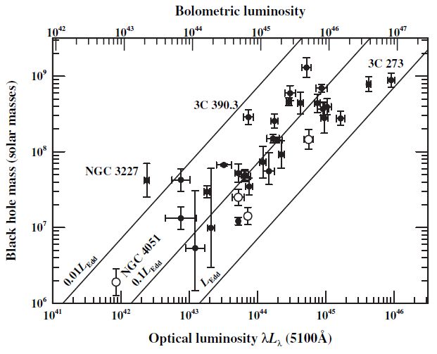Figure 9. The mass–luminosity relationship for reverberation-mapped AGNs. The luminosity scale on the lower x-axis is log λ Lλ in units of ergs s-1. The upper x-axis shows the bolometric luminosity assuming that Lbol ≈ 9 λ Lλ (5100 Å). The diagonal lines show the Eddington limit LEdd, 0.1 LEdd, ad 0.01 LEdd. The open circles represent NLS1s. From [25]