

One of the oldest and most challenging problems in astronomy is the measurement of distances to any astrophysical object on the sky. Although this task appears to be very basic in theory, it represents a major challenge in practice.
Aristarchus of Samos (310-230 BC) is probably the first astronomer to measure the distance between the sun and moon using trigonometry. In 265 BC he estimated the angle between moon-earth-sun at the point where the moon is exactly half full to 87°. Using the relation r / R = cos 87°, with r and R being the distance to the moon and sun, respectively, the distance to the sun should be 19 times the distance between earth and moon. Today we know that the exact angle is only sightly different (89.85°). However, not surprisingly the effect on the derived distance is huge, with the distance of the sun from the earth being 390 times the distance between earth and moon. Several other Greek astronomers, like Eratosthenes, Hipparcos, and Ptolemy, not only continued to measure the sizes of the earth and moon but also estimated the relative distances to the planets as far out as Saturn.
1.2. Important Steps Towards the Cosmological Distance Ladder
Significant advances regarding the astronomical distance scale had to await the 16th century, where Nicolaus Copernicus (1473-1543) introduced for the first time almost correct relative distances of the planets from the sun. In 1672, John Flamsteed (1646-1719) and independently Giovanni Domenico Cassini (1625-1712) measured the distance between the earth and sun to ∼ 140 million km and underestimated this distance only by 7%. At the same time, Sir Christopher Wren (1632-1723) proposed that nebulae might be distant star systems with the light of their individual stars being blurred into a milky, continuous glow (the ‘island universes’ theory of nebulae). However, it took until the 20th century to take the next important step concerning the distance scale in establishing the distance to these (extragalactic) spiral nebulae through the discovery and application of variable Cepheid stars in the Magellanic Clouds (MCs) by Henrietta Swan Leavitt (1868-1921). Harlow Shapley (1885-1972; Shapley 1919) investigated Milky Way Globular Clusters (GCs) and measured their distance with pulsating Cepheid stars that were calibrated using the Period-Luminosity (P − L) relationship for galactic Cepheids as established by Leavitt (1908). Assuming that the GCs are part of our own galaxy with an increased concentration towards the direction of Sagittarius, Shapley concluded that the central core of the Milky Way must be towards Sagittarius too. This correct picture, though having a wrong diameter for the Milky Way (100 kpc) due to underestimation of the contribution of interstellar extinction (dust), yielded in 1920 to the famous great debate between Heber Doust Curtis (1872-1942) and Harlow Shapley. Heber Curtis, himself a strong supporter of the ‘island universe’ theory, resolved individual stars in spiral nebulae that have created novae and concluded from a comparison with novae in our own galaxy that the novae in spiral nebulae need to be located far away. The final evidence that spiral nebulae are extragalactic systems was given later by Edwin Powell Hubble (1889-1953; Hubble 1926). Using new Cepheid discoveries, that were calibrated to Leavitt's P − L relationship of galactic Cepheids, he showed that M31 and M33 were far more distant than the Milky Way. Additional support was provided by Robert Julius Trümpler (1886-1956), who discovered the extinction to open (galactic) star clusters, and Vesto Malvin Slipher (1875-1969), who from 1912 onwards measured radial velocities of spiral galaxies with large recession velocities from the Doppler speed of spectral lines. In 1929, Hubble found a linear correlation between the apparent distances of galaxies d and their recession velocities vpec of form vpec = H0 · d (also called the Hubble law, Hubble 1929, see Section 3.3). The convincing conclusion that there indeed exists a relation between redshift and distance was given two years later using new observational data (Hubble & Humason 1931). However, this major advance in understanding did not suggest an expansion of the universe per se. The hypothesis of an expanding, homogeneous and isotropic universe that is still valid today was introduced with the mathematical works of Aleksandr Friedmann (1888-1925), Georges Lemaître (1894-1966, Lemaître 1927), and Howard Percy Robertson (1903-1961) who all contributed independently to the classical solution of the Einstein field equations. Using the Hubble law and the assumption that the expansion of the universe was slower at earlier times, the age of the universe today should be 1.8 Gyr and the Hubble constant H0 = 450 km s−1 Mpc−1.
With the application of new or improved techniques in measuring distances to extragalactic objects, the extragalactic distance scale was subsequently extended to larger distances. Walter Baade (1893-1960; Baade 1944) was the first to separate the stellar populations of spiral galaxies and GCs and derived a much smaller H0 of 250 km s−1 Mpc−1. Allan Rex Sandage (1926-2010) discovered that the ‘bright stars’ seen by Hubble are actually HII regions that consist of star groups and clouds of ionized hydrogen. Sandage's H0 of ∼ 75 km s−1 Mpc−1 corresponds to an age of the universe of ∼ 13 Gyr. For a recent progress report on measuring the Hubble constant to a precision of 5% using the most accurate distance indicators, the reader is referred to Freedman & Madore (2010), whereas observational probes to constrain the cosmic acceleration are presented in Riess et al. (2011) and Weinberg et al. (2012).
Figure 1 displays the extragalactic distance ladder with the most important standard candles in astronomy. The distance increases logarithmically from bottom to top, starting with our Milky Way, across the Local Group (LG) and extending towards the Local Super Cluster (LSC). Each technique represents an individual step in the distance ladder that is calibrated with a previous method of less-distant objects. The ultimate goal is a precise measurement of the Hubble constant that also gives information about the adopted galactic luminosity function and allows us to test models for dark energy (see also Section 7).
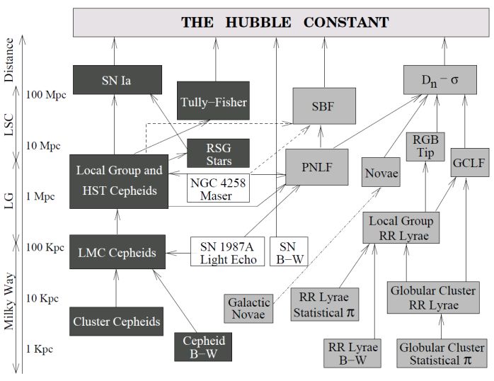 |
Figure 1. The extragalactic distance ladder. The dark boxes represent techniques useful in star-forming stellar systems (young Population I stars), grey-filled boxes denote methods that can be applied to quiescent stellar systems (evolved Population II stars), whereas open boxes give distance determinations using geometric techniques. Less-certain calibration steps are indicated as dashed lines. The distance increases logarithmically from bottom to top. Due to space constraints, the following abbreviations have been used: Baade-Wesselink method (B-W), Globular Cluster Luminosity Function (GCLF), Local Group (LG), Local Super Cluster (LSG), Planetary Nebula Luminosity Function (PNLF), Red Giant Branch (RGB), Red Super Giant (RSG), Supernova (SN), Surface Brightness Fluctuations (SBF), Parallax (π). The figure was adapted from Ciardullo (2006). |
Early attempts in the field of Surface Brightness Fluctuations (SBFs) were conducted by Baade (1944), who resolved Population II stars in galaxies of the Local Group. Individual star fluxes in external galaxies constitute a significant part of the stellar luminosity function of red giant stars and yield, besides the distance of the galaxy, substantial information on the stellar populations. Soon thereafter, Baum & Schwarzschild (1955) obtained observations of M31 and M32 (NGC 205) close to the limit of the resolution (historically called ‘incipient resolution’) and investigated their stellar populations using the ratio of the number of resolved stars to the total integrated light (the so-called ‘count-brightness ratio’). The empirical ratio of N / LV,tot is a useful proxy because it is sensitive to differences in the average stellar populations. The brightness was expressed in terms of visual (V-band) luminosities, but is in principle applicable to all wavelengths. Other works in similar directions followed. Mould et al. (1983; 1984) found similar luminosity functions for the dwarf ellipticals NGC 147 and NGC 205, whereas Pritchet & van den Bergh (1988) and Freedman (1989) measured the tip of the red giant branch via colour-magnitude diagrams for M31 and M32, respectively. However, individual stars can only be resolved for galaxies within the Local Group, thereby limiting the power of distance measurements considerably. Unfortunately, this restriction will not significantly change with the introduction of the next generation of large telescopes, see further Section 8. Nevertheless, this problem of measuring individual star fluxes without resolving them can be bypassed if a characteristic flux of a stellar population is determined. For example, for the red populations of globular clusters this average characteristic flux can be best measured at the bluest wavelengths where the red fluctuations are smallest. An alternative way to derive fluctuation amplitudes is by using a histogram of pixel amplitudes (Baum 1986, 1990). This statistical analysis of pixel brightness variations is a variant of the ‘count-brightness ratio’ method and can be used to establish the upper end of the Hertzsprung-Russell diagram and through a match between simulations and real data can estimate distances as far as the Virgo galaxy cluster.
In the late eighties, Tonry and Schneider invented a new way to quantify and measure surface brightness fluctuations to determine extragalactic distances (Tonry & Schneider 1988). The basic technique of SBFs consists of spatial pixel-to-pixel brightness variations, so-called fluctuations, which arise due to the varying number of stars within the pixels in a high signal-to-noise-ratio (S / N) Charge-Coupled Device (CCD) image of a stellar system, like a (globular) star cluster or an early-type galaxy or spiral bulge. The details of the theory and the basics of the method are described in Section 2.
Over the past decades, several articles have discussed some aspects of the SBF technique (e.g., Tonry et al. 1990; Tonry 1991; Jacoby et al. 1992; Tonry et al. 1997). However, there has been only one review on the subject, which concentrated mainly on the I-band (Blakeslee et al. 1999).
This article presents an updated critical review of progress in the application of the SBF method. In particular, the present work focuses on new developments in this field, like the use of near-infrared (NIR) photometric bands or recent theoretical model improvements. The article is organised as follows. In Section 2, the origin and technique of surface brightness fluctuations is explained in detail. Section 3 gives a short overview of observational attempts in determining SBF distances from both the optical and NIR perspectives. Selection effects and biases that may alter the accuracy of the SBF method and the application of SBF as a distance indicator are presented in Section 4. In Section 5, SBFs are discussed from a theoretical point of view. Further, this section describes the recent progress obtained in stellar population synthesis modelling. An alternative way of calibrating SBF observations is presented in Section 6. Concluding remarks are drawn in Section 7. Finally, Section 8 outlines some forecasts for the future.