With the Gaussian, when you go to maximize the likelihood

you discover that you must minimize the sum of the squares of the
residuals. This leads to
a very simple and straightforward set of simultaneous linear
equations. With the Lorentz function, you get

Try differentiating the right side of this equation with respect to each
of the unknown
parameters, and see where it gets you. Pretending that the error
distribution is Gaussian even if it isn't makes life a lot simpler.
The fact is, with real data you don't know what the probability
distribution of the errors
is, and you don't even know that it has any particular mathematical form
that is consistent
from one experiment to another. Most likely, some formula like the
Lorentz function - with
a well-defined core and extended wings - is a more reasonable
seat-of-the-pants estimate
for real error distributions than the Gaussian is, because the
Gaussian's wings fall off very
quickly. As I said, we all know that two- and three-sigma residuals are
far more common
in real life than the Gaussian would predict. This is because a real
observation is likely to
contain one or two large errors in addition to a myriad of tiny ones.
For instance, say you are doing photometry, with either a photomultiplier or a
CCD. During a ten-second integration things like photon statistics and
scintillation in the
atmosphere represent a very large number of tiny, quasi-independent
errors. According to
the Central Limit Theorem, these should indeed tend to add up to an
error distribution
which is very well approximated by a Gaussian. However, you also have
the finite chance
that a wisp of cloud, or a flock of birds, or the contrail of a jet
could pass in front of your star
while you are observing it. With a photomultiplier, the telescope
tracking might be erratic,
occasionally taking the star image closer to the edge of the aperture,
thus causing some
random amount of light to be lost. Or, if you are doing CCD photometry,
an unrecognized
cosmic ray could land on top of one of the star images in your CCD
frame, or the night-sky
fringe pattern might not subtract cleanly. It is even possible that
round-off error in
your equipment could contribute a significant part of the difference
between the "true"
and observed values of your measurement. In short, when you have many
very small,
independent sources of error which are all added up, yes, the total
error should be very
close to the Gaussian distribution. But if in addition to those tiny
errors, you also have
several potential sources of large random errors, one of the fundamental
postulates of the
Central Limit Theorem is violated, and there is no guarantee that the
final error distribution will be driven all the way to a Gaussian.
When an observation can possibly contain one or a few large errors, the error
distribution is not necessarily even symmetric. For instance, if we go
back to the photometry
example, if you think the sky is clear but in fact there are scattered
wisps of cloud which
occasionally pass in front of the telescope, the cloud will always make
the star you happen
to be observing at the time appear fainter. The clouds are presumably
just as likely to affect
your observations of standard stars as of program stars, so in the mean
the photometry is
still good. However, if the wisps of cloud occupy less than exactly 50%
of the sky, there
will be a systematic bias: you will tend to measure any given star
either a little too bright
(compared to the mean) or a lot too faint; if the wisps occupy more than
50% of the sky
it will be the other way around. If you occasionally forget to check
that the telescope is
looking straight out of the slit, so that once in a while the dome
covers part of the telescope,
or if there is a periodic tracking error which makes the star move near
to the edge of the
aperture for one second out of every 60, one ten-second integration out
of every six will
be a lot too faint, while the other five integrations will be a little
too bright, compared
to the average. In the case of CCD photometry, when a cosmic ray lands
on top of a
star image it will always make the star appear brighter, but when it
lands in a clear-sky
region, it may be recognized and ignored. Since there is no law of
Nature which says that
unrelated phenomena which preferentially produce positive and negative
errors must always
absolutely balance each other, you can see that real-world observational
errors do not only
limit the precision of our results, they can often introduce a
systematic bias as well. This
means that you must always be on the lookout for large residuals, and
you must be ready to do something about them.
Of course, you all know what to do with a bad measurement: you reject
it. You leave
the bad data point out of the solution and fit your model to the rest of
the points. Most of
us know a bad datum when we see it, but if we want to be scrupulous
about it, we will set
some limit, for instance three times the standard error, and feel good
about rejecting the
point if its residual is larger than that limit. If you are a truly
honest person, when you
publish the paper you will include the bad data point in your plots, but
will explain that
you omitted it when you computed the fit. Of course, you will feel best
about rejecting a
bad piece of data if you have some other reason to think that it is bad:
for instance, if you
encounter a discrepant measurement while reducing some photoelectric
photometry, and go
back to your observing log to discover that you had written "dome may
have been in the
way," you would feel perfectly happy to reject the discordant
observation. However, if a
data point is discrepant enough, you will discard it even if you have no
independent reason to suspect it.
What if you don't? Suppose you try to be completely honest and use every single
datum, discordant or not? Well, to illustrate what can happen, I ran
some more simulations.
This time the goal was to compute an estimate of the mean value of some
variable from
ten independent observations, where each observation has some finite
probability of being
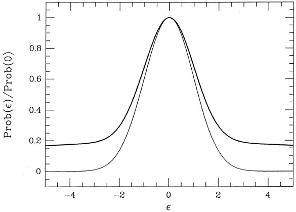
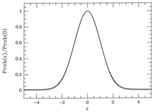
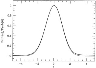
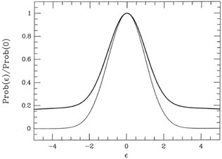
"bad." For the first test, I gave each observation a 90% chance of being
"good," which
meant that the observation was chosen at random from a Gaussian
distribution with mean
zero and standard deviation unity; the other 10% of the time the
observation was "bad,"
which meant that it was chosen at random from a Gaussian distribution
with mean zero
and standard deviation 10. Fig. 3-9
illustrates this probability distribution (heavy curve),
and compares it to a true Gaussian distribution with
 = 1 (light curve). As you can
see, when these two distributions are scaled to the same peak value it's
very hard to see
that the error distribution of my "observations" is non-Gaussian. Under
these conditions, I
generated 2,000 different sets of data, each set consisting of 10
independent variables chosen
from this composite probability distribution;
Table 3-1 contains five
typical lists of "data," where the "bad" ones are marked with asterisks.
= 1 (light curve). As you can
see, when these two distributions are scaled to the same peak value it's
very hard to see
that the error distribution of my "observations" is non-Gaussian. Under
these conditions, I
generated 2,000 different sets of data, each set consisting of 10
independent variables chosen
from this composite probability distribution;
Table 3-1 contains five
typical lists of "data," where the "bad" ones are marked with asterisks.
|
| Figure 3-9.
|
I initially calculated the mean of each sample of ten in two ways: (1)
knowing which
data were good and which were bad, and weighting them accordingly, and
(2) not knowing
which data were good and which were bad, and weighting them all
equally. Since neither the
"good" data nor the "bad" data are biased (both were selected from
probability distributions
with mean zero), we would expect that the means of the samples of ten
will scatter
symmetrically about zero. However, how closely they scatter about zero
will tell us how
good our estimator of the mean is. Thus, by looking at the standard
deviation of the 2,000
means generated by each of these two schemes, we can see how good that
scheme is at
coming up with the "right" answer. The 2,000 means generated with the
first scheme - that
is, perfect knowledge of which data were good and which were bad - was
0.3345; the
2,000 means generated with the second scheme, that is, no a priori
knowledge of which
data were good and which were bad, but treating all equally, was
1.042. The ratio of the
squares of these numbers - the ratio of the weights of the results
produced by the two
schemes - is 9.7. Call it 10. The second scheme produces results that
have lower weight,
by a factor of ten, than the first scheme. That means that by blindly
including every single observation, whether good or bad,
we have lost 90% of the weight of our results! Ninety
percent of the effort of collecting the data has been thrown away simply
by including that
10% of the data which happens to be of poor quality. We might as well
have gotten one
night of observing time and reduced that one night carefully, instead of
getting ten nights of time and including the bad results with the good.
Table 3-1. Five samples of random test
data
|
| | 0.30 | -4.85* | 0.16 | -0.14
| 3.96*
|
| | -0.49 | 0.23 | 0.76 | -0.19
| 2.02
|
| | -0.14 | 0.05 | 0.14 | -0.23
| -0.16
|
| | -0.14 | 0.15 | 3.82* | -7.48*
| -0.19
|
| | 1.06 | -1.77 | 0.67 | -0.39
| 0.87
|
| | -2.71 | 6.48* | -0.11 | 20.67*
| -1.08
|
| | -0.35 | -1.00 | -0.34 | -1.24
| -0.54
|
| | -1.56 | 0.84 | 1.99 | 0.77
| -0.21
|
| | 0.85 | -9.65* | -0.25 | -1.33
| -2.35
|
| | -0.16 | -0.21 | 2.18 | -7.84*
| -1.31
|
| CORRECT weights | -0.33 | -0.25 | 0.58
| -0.38 | -0.32
|
| ASSUMED weights | -0.33 | -0.97 | 0.90
| 0.26 | 0.10
|
 = 2, = 2,
 = 2 = 2 | -0.20
| -0.29 | 0.61 | -0.55 | -0.25
|
|
That factor of ten is not some accident; you can demonstrate from first
principles that
that is what you should have expected. Remember my statement in the
first lecture that
when you do properly weighted least squares (obtain the mean, in this
case) the weight of the
result is equal to the sum of the weights of the individual
observations? Well, even though for
this experiment any given set of ten data points could contain either no
"bad" observations, or one, or two, or ..., or ten, the typical set of
ten will contain nine good observations and
one bad one. So the typical set often will have total weight
(9) . (1) + (1) . (1/100) = 9.01, which
implies a standard error of 1 /
 9.01 = 0.333 for the weighted
mean. If we had left the bad
data out altogether and just averaged the good ones, we would have
gotten a typical total
weight of 9.00 - thus the bad data contribute practically nothing to a
properly
weighted mean. For the equal-weighted mean, however,
9.01 = 0.333 for the weighted
mean. If we had left the bad
data out altogether and just averaged the good ones, we would have
gotten a typical total
weight of 9.00 - thus the bad data contribute practically nothing to a
properly
weighted mean. For the equal-weighted mean, however,
propagation of errors tells us we should expect
which implies a standard error of 1.044 for the mean. So, as you can
see, the factor of ten
difference in total weight between the two schemes for computing the
mean is no accident, it is what I should have gotten.
Unfortunately, in real life we don't usually know ahead of time which
observations are
good and which are bad. We can't use the first scheme, and weight every
point properly.
The most we can hope for is to approximate the first scheme by reducing
the weights of
those data points which, after the fact, appear likely to be members of
the "bad" category.
This is why you must be prepared to employ (carefully!) some
weight-reduction scheme to
make the best possible use of your precious telescope time, if there is
any chance at all that
your error distribution might be non-Gaussian (practically always). I
would like to deny
that this necessarily constitutes "fudging," or "cooking" your
data. Provided that you are
intellectually honest, that you think carefully about what you are
doing, and that you tell
the referee and the readers of your paper exactly what you have done,
this is a legitimate
and necessary method for not wasting most of your effort by mixing in
extra noise in the form of poor observations.
The problem of exactly how you deal with bad data is especially
important in modern
astronomy, for two reasons. First, as I said a while ago we know that
some fraction of any
set of quantitative observations is going to be affected by occasional
large observational
errors for reasons that we can't always figure out. For instance, we
know that cosmic-ray
events will appear at unpredictable locations in CCD images and they
will have unpredictable
energies, that the night sky can flicker erratically, and that flocks of
birds can fly overhead.
With large modern data sets, I suspect that you will virtually always
find that the error distribution is significantly non-Gaussian (cf.
Fig. 3-9: it's non-Gaussian at the factor often
level!) Second, these large astronomical data sets are almost always
analyzed by computer,
and the stupid machine doesn't have any common sense. If you tell it to
add up a list of
numbers and divide by N, it'll do it. The computer won't see anything
odd about the data
set 0, -1, 3, 1, -2, 31927, 0, 1 - it'll add `em up and divide by
eight. You can spoil a lot of
good data this way. Instead, the computer programmer must imagine ahead
of time what
the possible problems could be, and must come up with purely numerical
ways of diagnosing
and dealing with these problems, so they can be understood even by a
dumb computer.
Of course, the easiest thing to do is to tell the computer to compute
the mean, check
to see whether any of the data points are away off in left field, and
recompute the mean
without the oddballs. This method is easily applied to more general
least-squares problems,
and fits right in with those reductions where you have to iterate
anyway, whether because
the equations are non-linear or because you have to deal with
observational errors in more
than one dimension. Unfortunately, the simple notion of simply rejecting
any datum which
looks bad is often unreliable, and in fact it involves some profound
philosophical difficulties.
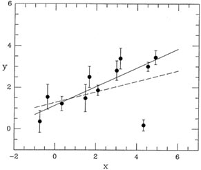
To understand what I mean, consider the task of fitting a straight line
to the data
shown in Fig. 3-10; the dashed line
represents the least-squares solution you would get if
the obviously "bad" point were included in the fit with its full natural
weight, and the solid
line is the answer you'd get if the bad point were arbitrarily given
zero weight, i.e., if it
were discarded. Suppose you had told the computer to derive a
least-squares fit using all
the data, and then to repeat the fit after rejecting any data point
whose residual from that
first fit was greater than five standard deviations. Now, suppose that
this data point is
precisely 4.999 standard deviations away from the dashed line. So
everything's hunky-dory:
the point is within 5 of the
solution, and the dashed line is what you get. But now suppose
that the point was only a tiny little bit lower, so that it was 5.001
standard deviations from
the dashed line. The computer, following your instructions, would first
produce the dashed
line as the provisional solution to your problem, then it would see the
spurious datum and
reject it, then it would compute the solid line as the correct solution,
and that's the answer
you'd submit to the journal. In other words, by making a tiny change in
a single data point
- and that data point already highly suspect to any sensible human
observer - you've made a big change in your final answer. This is
Not Good.
|
| Figure 3-10.
|
If this problem were not a simple linear least-squares fit of a straight
line, but rather
were a non-linear problem or a two-error problem where you had to make
an initial starting
guess and then iterate to a solution, you'd run into another paradox. If
your first guess at
the correct straight line lay somewhere below the data, then the
discrepant point would be
within 5 of the provisional
answer, and the solution would eventually
settle down - after
some iteration - at the position represented by the dashed
line. Conversely, if your initial
guess at the solution lay generally above the data points, since the
discrepant data point
was more than 5 from the
provisional solution, the computer would reject it early, and
the solution would happily converge to the position of the solid
line. In other words, you
could get two very different answers out of the same data set, depending
upon your crude,
initial starting guess at the solution. This is also Not Good.
So I've pointed out two major problems with simply telling a dumb
computer to reject
any data point that lies too far from a provisional solution: you can
get big changes in
the answer from tiny changes in a single datum, and you can get big
changes in the final
answer by making different starting guesses. If a human being were
plotting the data and
sketching the curve, no problem: some reasonable compromise would
suggest itself. It turns
out that you can get the computer to compromise, too - automatically and
without human
supervision - once you recognize the problem. Let the machine exercise a
little healthy
doubt. Mathematically speaking, what I mean is we should empower the
computer to apply
partial weights to apparently discrepant observations. In particular,
once a provisional
solution as been generated, any observation with a residual << many
would be assigned
its full 1 / 2
natural weight, while an observation with a
residual >> many would be given
a much smaller weight than it would nominally deserve. On this basis a
new solution would
be computed, new residuals derived, new weights assigned, and so on,
until a consistent, repeatable answer was achieved.
So let's rerun our little thought experiment with this scheme in
place. The computer fits a straight line to the data in
Fig. 3-10, with each point receiving
its full, natural, 1 / 2
weight, and the dashed line results. The computer then sees one data
point lying way off
the provisional fit, and repeats the solution giving that point, say,
half weight. The new
least-squares line lies about half-way between the dashed and solid
lines, and the discrepant
point now lies a little bit farther from the current provisional fit. So
the computer reduces
its weight still more, let's say to 0.4 times its natural weight. The
provisional fit moves up
just a whisker more, and soon settles down between the solid line and
the dashed line, but
closer to the solid line, with the computer ultimately assigning the
oddball point maybe 0.38
times its natural weight. Move the discrepant point up or down by a bit
and the solution hardly changes.
Now let's see what happens with the iterated nonlinear reduction. If our
starting guess
is somewhere below the bulk of the data points, the discrepant point
will start off with a
comparatively high weight, but the other points will still tend to pull
the solution up. The
weight of the discrepant point will be reduced, and the solution will
continue to move up,
eventually settling down somewhere just below the middle of the bulk of
the data points.
On the other hand, if the starting guess were somewhere above the data
points, the weight
of the oddball would start out low. But as the other data pulled the
solution down, the
oddball's weight would increase, and the solution would once again
settle down somewhere
just below the middle of the bulk of the data points - at exactly the
same place as before.
Now don't get me wrong. I'm not saying that the answer this
scheme gives you is
the "right" solution; I'm not saying that it's the "best" solution; I'm
only saying that it's
a consistent, repeatable solution which is robust against both small
changes in individual
data points and large changes in the starting guess. It keeps the idiot
computer from being
satisfied with some non-unique answer. If you were drawing a smooth
curve through data
points by hand, you wouldn't need a scheme like this: you'd realize that
the oddball point
was a little iffy, and would concentrate on making sure the curve
described most of the data
well. A computer just isn't this smart all by itself. When you do a
photometric reduction of
a CCD frame, the computer is solving thousands of little least-squares
problems; for a single
observing run, there may be hundreds of thousands or millions of
least-squares problems. A
scheme which teaches the computer to be less influenced by discrepant
data may allow you
to get a few pretty good answers when otherwise you would have gotten
garbage. In fact, I
think I'll go out on a limb and argue that when you don't know what the
true probability
distribution of the observational errors is, you only know that it
probably isn't Gaussian,
there is no such thing as the "right," or "best" answer; a consistent,
repeatable, robust answer is the very most you can hope for.
There are only a few things that you want to be sure of, for logical
consistency and
simplicity. (1) Points with residuals small compared to their standard
errors should get
something approaching their full natural weight. Let me use
f( ) to
represent the fudge-factor by which the weight of an individual data
point is changed on the basis of the size of
its residual. Now the weight that the point is actually assigned is
given by wi =
f(i) /
i2
(let's just say the scaling factor s = 1, shall we?), and we want
lim->0 f =
1. (2) Really,
really bad points should have weights approaching zero:
lim->
) to
represent the fudge-factor by which the weight of an individual data
point is changed on the basis of the size of
its residual. Now the weight that the point is actually assigned is
given by wi =
f(i) /
i2
(let's just say the scaling factor s = 1, shall we?), and we want
lim->0 f =
1. (2) Really,
really bad points should have weights approaching zero:
lim-> f = 0. That way, you
know it doesn't matter whether the oddball has a
100 residual or a
200 residual, you'll
get essentially the same answer in either case. In fact, if you consider
the condition for a minimum of
f = 0. That way, you
know it doesn't matter whether the oddball has a
100 residual or a
200 residual, you'll
get essentially the same answer in either case. In fact, if you consider
the condition for a minimum of
 2,
2,
you can see that you really want f to fall off at least as fast
as -1; otherwise
the really
humongous blunders will continue to distort the solution more the larger
they get. (3) The fudge-factor f should be a monotonic, gradual,
smooth function of ||,
or else you'll get
back into the paradoxes: small changes in a datum (changes which would
move across a
discontinuity in f) would produce discrete changes in the solution, and
different starting
guesses might converge to different stable points, where one solution
generates values for
f which reproduce that solution, whereas another solution would generate
different values for f which would reproduce
that solution.
If f is sufficiently gradual and continuous, this won't happen.
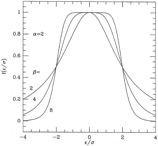
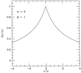
For some years now, I have been using one particular scheme meeting the
above criteria,
which has turned out to be handy in a wide variety of applications:
where and
are two constants
which can be set so as to fine-tune the machinery to a
given application. Fig. 3-11 shows three
functions f, for = 2
and =
2, 4, and 8. If you
study the equation and the figure, you'll see that this formula does
indeed go to unity for
small and to zero for
large , and as long as
 1 it will fall off
at least as fast as -1
for large . You may also
ascertain that represents the
half-width of the function: any observation whose residual is
times its standard error will be
assigned half its natural
weight. Finally, note that in the limit of very large
, this scheme
degenerates to the old,
classical, reject-any-observation-whose-error-is-larger-than-some-limit:
as ->
1 it will fall off
at least as fast as -1
for large . You may also
ascertain that represents the
half-width of the function: any observation whose residual is
times its standard error will be
assigned half its natural
weight. Finally, note that in the limit of very large
, this scheme
degenerates to the old,
classical, reject-any-observation-whose-error-is-larger-than-some-limit:
as ->

|
| Figure 3-11.
|
There is one case which is worth special mention:
= 1. This is
illustrated in Fig. 3-12. It
looks a bit odd, but to understand what is neat about this
fudge-function, reconsider the sum
For >>
,
cancels out. This means
that, all other things being equal, any large residual
contributes exactly the same amount to this sum as any other, only the
sign of the residual
being retained. By making a comparatively small, we can make our
solution depend upon
making the number of positive residuals equal the
number of negative residuals (scaled, of
course, for the weight of each point and the sensitivity of the fitting
parameter to each point),
regardless of the size of those residuals. In other words, we now have a
mechanism which
permits us to do a least-squares-like analysis, possibly with an
equation which is nonlinear
in the parameters, possibly with data possessing errors in more than one
dimension, which
finds a solution passing through the weighted median of the data rather
than through the mean. This can be really handy with really cruddy data.
|
| Figure 3-12.
|
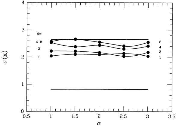
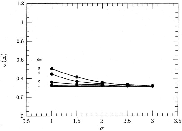
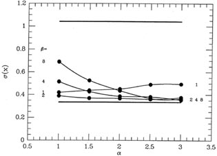
Yes, yes, yes, but does it work? Well, I reran the reductions of the
same 2,000 sets-of-ten
as before, again without using any a priori knowledge of which
observations were "good"
and which were "bad," but this time using my weight-fudging scheme to
reduce the impact
of data points whose extreme values made them appear somewhat
suspect. Representative
means derived with = 2 and
= 2 are shown on
the last line of Table 3-1. In
Fig. 3-13
I have plotted the standard deviation of the 2,000 fudged means as
derived from various
values of and
. The horizontal
line at = 0.33 represents the
standard deviation of
the means achieved with perfect knowledge of which points are good and
which are bad,
and the horizontal line at =
1.1 represents the standard deviation obtained with a blind,
weight-'em-all-the-same attitude. As you can see, the quality of the
answers that you get
with my automatic reweighting scheme is surprisingly insensitive to
which values of and
you adopt. Under
the hypothesized circumstances, with one point in ten being a factor
of ten worse than the rest, by using intermediate values of
and
(setting each of them
to somewhere around 2 or 3) you get marginally better results, on
average, than with more
extreme values. It's also pretty obvious that while this reweighting
scheme is never as good
as having Perfect Knowledge of Reality, it's a darn sight better than a
stubborn insistence
on treating all the data equally, no matter how odd they may seem.
|
| Figure 3-13.
|
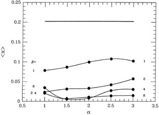
How does my gimmick work under other circumstances? To find out, I ran some
more simulations, of course. Suppose there is a preferential bias among
the "bad" data
points? For my second test, I assumed as before that the probability of
getting a "good"
measurement was 90%, where again a good measurement had mean zero and standard
deviation unity; this time, however, the 10% of "bad" measurements were
assigned mean 2
and standard deviation 5. Fig. 3-14 shows
this probability distribution as a heavy curve and,
as before, the light curve is a genuine Gaussian probability
distribution with = 1, which
has been scaled to the same peak value. Again, the difference between
the "true" probability
distribution for my "observations" and a Gaussian is slight, and would
be impossible to
detect in any small sample. The bias in the "bad data," in particular,
is barely detectable.
In this test a "correct" answer of 0.0 for our hypothetical physical
quantity is what we want
to get from our data. Unlike in the previous test, in this one we can
use both the mean
of the 2,000 answers and their standard deviation as different measures
of the quality of
the weighting scheme: the mean of the answers will show the extent to
which the bias in
the bad data points influences the accuracy of our answer, the standard
deviation of the
2,000 answers will show how the extra scatter in the bad points affects
the precision of the
result. When we use our Perfect Knowledge of the probability
distribution of each datum,
we can both correct the bad ones for their systematic bias and weight
them appropriately.
Therefore the expected mean of the 2,000 means would be 0.0, and we
expect those standard deviation of those 2,000 means to be
|
| Figure 3-14.
|
However, when we pretend we don't know which observations are good and
which are poor,
and blindly take the straight mean of all the data in each set of ten,
we get answers which average
Naively you'd expect a standard deviation
but, in fact, the bias in the "bad" data introduces additional scatter:
the possibility that
any given set of ten might have two bad data points, or three, or none,
makes the answers
scatter by more than their total weights would imply. I actually
observed ( ) = 0.647
for these 2,000 data sets. Now, when I turn on my magic reweighting
scheme with various
choices of and
, I get the means
represented in Fig. 3-15 by the big
dots connected by
smooth curves. As you can see, with a fairly severe clipping of the
apparently discrepant
data ( ~ 1.5-2,
~ 4-8) we can virtually
eliminate the systematic bias in the results:
the minimum value of <>, obtained
with = 1.5 and
= 4 is 0.0055 -
more than thirty
times smaller than the bias produced by accepting all data
blindly. Taking the "median" of
the data (actually, adopting my weighting scheme with
= 1 and
small which, as I said
earlier, shades the answer toward the median) offers the least help: it
reduces bias only by a
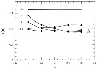
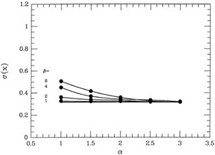
little over a factor of 2. The standard deviations of the 2,000 means
are shown in Fig. 3-16,
which suggests that the precision of the answers is optimized by a
somewhat more gentle
clipping than that yielding the best accuracy: values of
2,
2
yield ()
) = 0.647
for these 2,000 data sets. Now, when I turn on my magic reweighting
scheme with various
choices of and
, I get the means
represented in Fig. 3-15 by the big
dots connected by
smooth curves. As you can see, with a fairly severe clipping of the
apparently discrepant
data ( ~ 1.5-2,
~ 4-8) we can virtually
eliminate the systematic bias in the results:
the minimum value of <>, obtained
with = 1.5 and
= 4 is 0.0055 -
more than thirty
times smaller than the bias produced by accepting all data
blindly. Taking the "median" of
the data (actually, adopting my weighting scheme with
= 1 and
small which, as I said
earlier, shades the answer toward the median) offers the least help: it
reduces bias only by a
little over a factor of 2. The standard deviations of the 2,000 means
are shown in Fig. 3-16,
which suggests that the precision of the answers is optimized by a
somewhat more gentle
clipping than that yielding the best accuracy: values of
2,
2
yield ()
 0.36
(as compared to 0.33 for perfect knowledge of good and bad, and 0.65 for
an equal-weight reduction).
0.36
(as compared to 0.33 for perfect knowledge of good and bad, and 0.65 for
an equal-weight reduction).
|
| Figure 3-15.
|
|
| Figure 3-16.
|
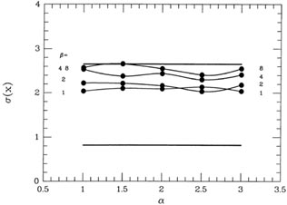
Well, suppose you make a serious mistake: suppose you think that your
measurements
are pretty good, but in fact most of them contain large random errors
from a source you are
unaware of? For my third experiment, I assumed that there was only a 30%
chance that
any given datum was "good" (mean zero and standard deviation unity) and
a 70% chance
that it was "bad" (mean zero and standard deviation 10; see
Fig. 3-17). Suppose you try
to reduce these data blithely assuming that every data point has
= 1, so that they all
get equal weight? Well, pretty obviously you're going to get means from
your sets-of-ten showing a standard deviation
For comparison, if you knew the actual standard error of each datum, the
very best you could hope for would be means showing a standard deviation
(Most groups of ten will have three or so decent observations; by
knowing which ones they
are and neglecting the rest - well, giving them the one one-hundredth
weight that they
deserve - you could come up with OK results. But we don't usually know
which ones are
good in real life, do we?)
(4) With data this badly corrupted, even my
reweighting scheme
can't perform miracles. But, as Fig. 3-18
shows, it is still better than blindly accepting
all data as of equal legitimacy. Of the weighting schemes I tried, the
pseudo-median is the
best. With = 1 - 2
and almost any value of , you
can get the standard deviation of the
means down to as little as 2.0. When compared to the "blind" standard
deviation of 2.65,
this represents a 32% reduction in the standard error or a 76% increase
in the weight of
your results. This is the same as getting seven nights of telescope time
for the price of four,
all through enabling the computer to feel some doubt about apparently
discordant data.
|
| Figure 3-17.
|
There is one more question which you must have answered before you will believe
that what I'm telling you is any good. "Suppose there is nothing wrong
with any of
my observations. How much honest information will I be throwing away by
telling the
computer to reduce the weight of any data point it doesn't like?" One
more simulation. This
time I gave each datum a 100% chance of being "good," with the same
normal, Gaussian
probability distribution with mean zero and standard deviation
unity. Again, I generated
2,000 data sets of size ten and took their means both without and with
my automatic reweighting scheme. The results are shown in
Fig. 3-19, and the answer
is, unless you use a truly vicious clipping scheme with very large
and very small
- so the computer
completely discards any data point which lies the least little bit away
from the mean of its group of ten - you lose very little. When
= 1 for
= 1 (so that, in
effect, your answer is the mean of those data less than
1 from the answer, shaded toward the
median of the rest)
the standard deviation of the 2,000 answers is 0.3265, as compared to
the "right" answer
of 0.3162 = 1 / 10 and things get
even better for larger . For
more a more intermediate
clipping scheme, =
2 and = 2.5, I find the
standard deviation of the answers is 0.3185.
This represents a 1.5% loss of information, as compared to using the
"right" observational
weights - the rough equivalent of throwing away one minute's observing
time out of every
hour. How many of us operate at 98.5% efficiency when performing a chore
for which we were not intended?
|
| Figure 3-18.
|
Please let me summarize my basic conclusions from the second half of
this talk. First,
unless you know with 100% absolute certainty that the distribution of
your observational
errors is Gaussian, and unless you know with perfect accuracy what the
standard error of
every one of your observations is, classical, standard,
look-it-up-in-a-cookbook least squares
does not guarantee you the best possible answer from your data. In fact,
with only a tiny
admixture of poor observations, you can destroy a great deal of
information. You must
remember to teach your computer to recognize grossly discordant data (as
in the data set
(0, -1, 3, 1, -2, 31927, 0, 1), which I used as an example
earlier). However, under some
circumstances (i.e., iterated non-linear or multi-error solutions)
telling the computer to
reject discordant data does not guarantee you a self-consistent,
repeatable answer from a
given data set. You can partially overcome these problems and improve
the consistency,
precision, and accuracy of your final answers by enabling the computer
to feel a healthy
skepticism about apparently discordant data. When I am reducing real
data, unless I have
an absolute conviction that the errors are Gaussian, completely
Gaussian, and nothing but Gaussian with known
's, I find that routinely applying my
reweighting scheme with
~ 2 - 2.5 and
~ 2 - 4 does my
iterated least-squares solutions a
whole lot more good, on average, than harm.
|
| Figure 3-19.
|
Does this mean that you can now feed your computer any kind of garbage and have
it give you back Truth? Of course not. Does this mean that the
astronomer no longer
has to look at his or her data? Of course not. An empirical reweighting
scheme like this
one offers you some insurance against non-ideal data, but it does
nothing to protect you
against fundamental paradigm errors. Your discordant data points may be
due not to wispy
clouds, flocks of birds, or cosmic rays; instead they may be heralding a
new law of physics.
Computers can't recognize this (at least, not yet), only trained
scientists can. In the next
lecture or two I plan to give you some practical data-reduction tasks
where my reweighting
scheme helps, but these are all cases where there is very little danger
of uncovering new
laws of physics. In short, I think it is still true that people who are
unwilling to think won't
do very good science, with or without computers. There is still no
practical substitute for
a thorough understanding of your material and some deep thinking about
its implications.
4 In fact, even knowing the weights
doesn't actually produce means this good. Samples
of size ten are not big enough for the Central Limit Theorem to drive
the probability
distribution for the mean of each sample to the Gaussian distribution,
when the distribution
for the individual observations is this strongly non-Gaussian. With an
average of three
"good" data points per sample of ten, there is a finite chance that any
given sample will
contain no good data. The means of such samples will typically be so far
from zero that
they will drive up the root-mean-square value of the means. I actually
observed 0.818 - rather
than 0.571 - as the standard deviation of my 2,000 means-of-ten,
assuming perfect knowledge of good and bad. Back.