


In my final two lectures I will discuss the general subject of Stellar Photometry with CCDs, and will talk in particular about ways in which statistics contribute to the subject - especially the sort of statistics that you can't find in cookbooks. But first of all let me deal with some more general, astronomical questions. Why do we do Stellar Photometry with CCDs in the first place? I'm not going to consider that part of the question which is "Why do we do stellar photometry?" - since we all know that stellar photometry is one of the very most exciting and important tasks of modern astrophysics - but I do want to answer that part of the question which is "Why do we do it with CCDs?"
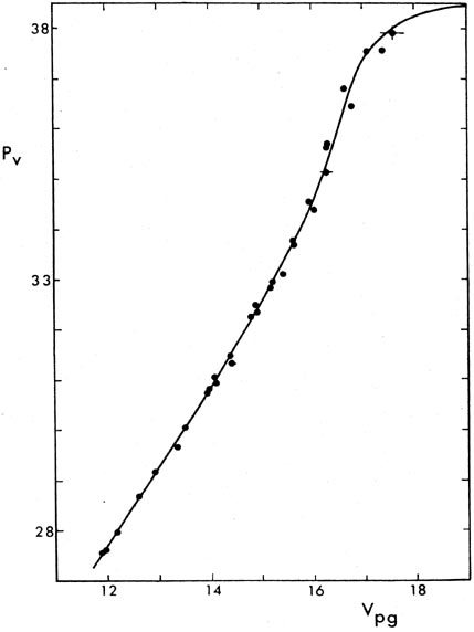
As you know, "CCD" stands for "charge-coupled device." These are small, solid-state arrays of silicon photodetectors which, when put at the focus of a telescope, enable us to obtain a digitized representation of a small portion of the sky. Fig. 4-1 is one of the best arguments I can present for why it's worthwhile to use these little dealybobbers for stellar photometry. The figure shows three different color-magnitude diagrams for the globular cluster 47 Tucanae. All three were constructed by the same astronomers using the same telescope, but with three different generations of image-detector technology. (The top parts of the three color-magnitude diagrams, that is, the cluster's giant and horizontal branches, are the same data in all three panels. What I want you to notice just now is the evolution with time of the bottom part of the diagram - the cluster's main sequence.) Rest assured that, in its day, each of these color-magnitude diagrams was considered one of the best and deepest that had ever been made. The left-hand panel is based on the "classical" technique of photographic photometry, where images of the cluster were recorded on photographic plates, and then a device called an iris photometer was used to measure the diameter and the blackness of each star image on those plates (Hesser and Hartwick 1977). Since photographic plates are rather non-linear recorders of relative intensity, these diameter and blackness measurements come out in some arbitrary units and on a varying scale. Thus, they can only be related to legitimate stellar magnitudes through measuring a number of stars on each plate whose brightnesses had previously been determined by photoelectric techniques. A example of such a calibration curve, from Stetson and Harris (1977), is shown in Fig. 4-2. Largely because of the extreme difficulty of obtaining adequate photoelectric observations for faint stars, photographic photometry was seldom reliable much below about 20th magnitude (and more recent work with CCDs has found serious systematic errors in a number of famous old studies at even brighter levels than this).

|
| Figure 4-1. |
|
| Figure 4-2. |
The middle color-magnitude diagram in
Fig. 4-1 was based on data obtained with a
SIT Vidicon camera
(Harris, Hesser,
and Atwood 1983a,
b). This device
used standard,
commercial television technology to obtain a digital image of a small
area of sky. One
of the great things about the Vidicon was that it combined the quantum
efficiency of a photocathode (~ 20%, as compared to
 1% for most photographic
emulsions) with the
plate's ability to record two-dimensional images. But also - perhaps
even more important
- to a reasonably good approximation the Vidicon was photometrically
linear, which means
that the signal produced by the detector was directly proportional to
the brightness of the source:
1% for most photographic
emulsions) with the
plate's ability to record two-dimensional images. But also - perhaps
even more important
- to a reasonably good approximation the Vidicon was photometrically
linear, which means
that the signal produced by the detector was directly proportional to
the brightness of the source:
This meant that the conversion from data numbers to instrumental
magnitudes did not require a full calibration curve, the way it did with
photographic plates; all you needed was
a single zero-point constant, which could be obtained from just the
brightest stars in the frame, or even from standard stars in other parts
of the sky if the night was photometric.
For both of these reasons (sensitivity and linearity) the SIT Vidicon
enabled astronomers to make color-magnitude diagrams extending one to
two magnitudes fainter than was practical
with photographic/photoelectric techniques. And they could do it in less
time, in part because of the combination of sensitivity with multiplex
advantage, but also because they
no longer had to combine two observing techniques (and two or more
observing runs) to
get their color-magnitude diagram: they could do it all at once.
Still, Vidicon cameras enjoyed only a very brief day in the sun (so to
speak), because
they were almost immediately supplanted by something even better:
CCDs. An early
(astronomically speaking) CCD made the rightmost color-magnitude diagram
in Fig. 4-1.
As I said before, CCDs are image detectors based upon solid-state
silicon semiconductor
technology. They can be somewhat bigger than Vidicons, having
photosensitive areas ranging from 1.2 cm on a side to
Before I go deeply into the subject of exactly how we do stellar
photometry with
CCDs, let me just briefly mention who does stellar photometry with
CCDs. Here is a list
of the most famous existing packages for photometry from two-dimensional
digital images
(I include only packages which are designed to deal with crowded-field
conditions, where
stellar images may overlap each other).
In most ways, for most typical applications, and as far as I know, these
programs are
roughly comparable in accuracy, convenience, and power. Any particular
program may
be less convenient or less accurate in some applications, while the same
program may
offer distinct advantages for other tasks. I do not intend to present
any value judgments.
Instead I will spend my time talking about DAOPHOT because that is the
program I am
most familiar with. You should not take this to mean that I think that
DAOPHOT is much
better (or much worse) than any of the other programs - I have many
opinions on this
subject, but I'm not planning to present any of them here and now.
There are numerous tasks which a computer program or ensemble of programs must
perform, in order to get from the digital image to a data table
containing standard
magnitudes and colors for a large number of stars. Today I will discuss
the first half of
the problem: the path from a single data frame to a list of positions
and stellar magnitudes
for the stars contained in that frame. Tomorrow I will discuss the
second half of the problem:
the path from a number of lists of positions and relative magnitudes
obtained from a number
of frames, to a single list of calibrated magnitudes and colors for the
stars in the field. I
will not discuss the problems of image-rectification: questions of bias
levels, dark signal,
flat-fielding and the like. Unfortunately, there have not yet been
enough studies done and
papers published in these areas, and I do not know of a good,
comprehensive, current,
essentially correct cookbook for dealing with everything that can go
wrong. Understanding
this subject seems to be still a matter of picking up a snatch of
information from this
paper, hearing a good idea from that astronomer over a glass of beer,
and figuring it out for
yourself. However, there's not enough time left to do everything, so I'm
leaving this stuff
out. Ask me over a glass of beer someday (you buy), and I'll tell you
what little I know of the subject.
So, here is today's list of data-reduction tasks to consider. I present
them in the DAOPHOT nomenclature.
First you must FIND the stellar-appearing objects in the frame. Each
program has its
own method - sometimes several methods - of performing this, but the basic idea
is to produce an initial list of approximate centroid positions for all
stars that can be
distinguished in the two dimensional data array. The star finder must
have at least
some ability to tell the difference between a single star, a blended
clump of stars, and a
noise spike in the data. It's a good idea to get a crude estimate of
each star's apparent
brightness at the same time. [For cognoscenti, this step combines
DAOPHOT's FIND
and PHOTOMETRY routines; these are discussed separately below.]
Next, the program must measure, encode, and store the
two-dimensional intensity
profile of a typical star image in the frame. Again, each package does
this in a different
way, but the one basic idea which is common to all packages is that the
shape of the
profile is assumed to be independent of the brightness of the
star. Therefore, the profile
shape can be determined from one or more bright, isolated stars, and
then this profile is
fitted by means of least squares to other program stars (which may or
may not overlap
with each other) pretty much as we did it in the second lecture.
So, obviously, step 3 is to fit the model profile obtained in step 2
to the images of the
stars found in step 1. Assuming that the shape of the profile of each
star is now known,
we must use nonlinear least squares to shift that profile in x
and y and determine
the local background intensity - which is the local diffuse sky
brightness - and the
intensity amplitude of the profile - which gives the relative brightness
of the star - to
best match the actual observed intensity data within the star
image. Since this is
a nonlinear problem, you need to have starting guesses at the fitting
parameters to
get the iterated least squares going; these come from step 1 above. In
real images
of astronomical starfields, the profiles of several stars will sometimes
(often? almost
always?) overlap by a bit. The reduction procedure must be able to
recognize this
situation and determine the positions and brightnesses of blended stars
simultaneously.
The next two generic tasks are not necessarily part of the "photometric
reduction"
procedure in the strictest possible sense of the phrase, but they are so
essential to
evaluating the results and demonstrating their quality to other people,
that any right-thinking reduction package includes them.
Once you have fit model profiles to all the stars in some
two-dimensional digital frame,
you want to subtract out these model profiles, so that you can examine
the fitting residuals by eye and/or software. This enables you to recognize
problems, such as stars
that the star-finding routine has missed, and galaxies or image flaws
that have been found and reduced as though they were stars.
Finally, once the model stellar profile has been determined, it is
extremely handy to
be able to add it back into the image at various locations and with
various intensity
amplitudes. This process creates images of additional "stars" whose
positions and
relative brightnesses are known a priori. By running this new frame
through the same
reduction procedure as the original one, the effectiveness and accuracy
of the star-finding
and profile-fitting routines can be checked with full quantitative rigor, under
the precise seeing, sampling, and crowding conditions relevant to your
study.
I wrote a computer program - DAOPHOT by name - which performs all of the
steps outlined above. Let me tell you something how it does them, and
why. (I would like
to repeat: this discussion is intended to exemplify ways in which least
squares and other
statistical methods can be employed in the field of stellar photometry
with CCDs, using
a software package that I am personally familiar with. If I don't give
equal time to your favorite package, tough.)
5 One obvious exception is large-area
survey work, such as with Schmidt telescopes for
example, where the enormous size of photographic plates (up to 50 cm
square, in current
astronomical applications) compensates for the loss of quantum
efficiency not to mention
the much greater ease of transporting and displaying the data.
Back.
 3 cm, as compared to
about 1 cm; they can be more
sensitive than Vidicons, reaching peak quantum efficiencies in the
neighborhood of 70%,
as compared to ~ 20%; and finally, they can be much more stable than
Vidicons, because
they consist of physical patterns permanently imbedded in a chunk of
silicon, while the
TV cameras rely on a scanning electron beam, with its propensity for
being bent by stray
magnetic fields or even by the electronic image which has built up on
the target. This
makes observations made with CCDs much more repeatable and easy to
calibrate. You can
easily see in Fig. 4-1 how the greater
sensitivity and stability of the CCD have enabled the astronomers
(Hesser, Harris,
VandenBerg, Allwright, Shott, and Stetson 1987)
to produce
a main sequence for 47 Tucanae which is both much deeper and much
narrower than was
possible with either of the two previous technologies. What a difference
a decade makes! It
is because the CCD is in almost every way the best existing detector for
obtaining optical images in astronomy
(5) that I call these two lectures
"Stellar Photometry
with CCDs," even
though most of the things I will have to say would apply equally well to
photometry obtained
from other types of photometricaily linear two-dimensional images.
3 cm, as compared to
about 1 cm; they can be more
sensitive than Vidicons, reaching peak quantum efficiencies in the
neighborhood of 70%,
as compared to ~ 20%; and finally, they can be much more stable than
Vidicons, because
they consist of physical patterns permanently imbedded in a chunk of
silicon, while the
TV cameras rely on a scanning electron beam, with its propensity for
being bent by stray
magnetic fields or even by the electronic image which has built up on
the target. This
makes observations made with CCDs much more repeatable and easy to
calibrate. You can
easily see in Fig. 4-1 how the greater
sensitivity and stability of the CCD have enabled the astronomers
(Hesser, Harris,
VandenBerg, Allwright, Shott, and Stetson 1987)
to produce
a main sequence for 47 Tucanae which is both much deeper and much
narrower than was
possible with either of the two previous technologies. What a difference
a decade makes! It
is because the CCD is in almost every way the best existing detector for
obtaining optical images in astronomy
(5) that I call these two lectures
"Stellar Photometry
with CCDs," even
though most of the things I will have to say would apply equally well to
photometry obtained
from other types of photometricaily linear two-dimensional images.
RICHFLD
Tody 1981
ROMAFOT
Buonanno, et
al. 1983
WOLF
Lupton and
Gunn 1986
STARMAN
Penny and
Dickens 1986
DAOPHOT
Stetson 1987