


A. Growth curves
To repeat myself redundantly, the first dirty problem relates to the fact that the magnitudes which come from profile fitting are purely relative magnitudes: they tell you how much brighter or fainter the program star is than the star(s) which defined the model profile for that frame, but they do not tell you the instrumental magnitude of each star in absolute terms. In order to find out how bright each program star really is, you need to know exactly how many detected photons are contained in the actual profile(s) of some star(s) in the frame. This number is then divided by the integration time to get the star's apparent flux in photons per second, which is converted into an instrumental magnitude on an absolute system by computing -2.5log(flux). The relative magnitude differences derived by the profile-fitting photometry then allow you to place all the program stars in the frame on the same external system. Finally, relying on the stability of the detector, you can transform these results to true magnitudes on somebody's standard system by comparing them to instrumental magnitudes obtained in the same way for standard stars, just as you would have done with data from a photomultiplier.
The problem here is the fact that the shape and size of a stellar image
are affected
by seeing, telescope focus, and guiding errors - any or all of which may
change from
one exposure to the next. Even if you write a profile-fitting photometry
program which
describes a frame's PSF with some analytic function, it is not
necessarily safe to assume
that you can simply integrate that function from minus infinity to plus
infinity in x and
y (or from zero to infinity in r), and call the result the
total number of detected photons
within the profile. In profile-fitting photometry, you adjust your
analytic model to obtain
the best possible representation of the core of the profile, where most
of the photometric
and astrometric information resides. If you want to be at all practical,
you are not likely to
include more than six or eight image-shape parameters in your analytic
star model. Once
these parameters have been adjusted to match the bright part of the
profile, there is no
guarantee that they will match the low surface-brightness, low
signal-to-noise-ratio wings
of the star image. Thus, when you come along and multiply this model
profile by 2  r dr
and integrate from zero to infinity, it's easy to believe that you might
make an error of a
few percent in the total volume under the profile. An error of a few
percent, of course, is completely intolerable.
r dr
and integrate from zero to infinity, it's easy to believe that you might
make an error of a
few percent in the total volume under the profile. An error of a few
percent, of course, is completely intolerable.
The easiest way to derive a consistent measure of the total number of photons contained in a star image is simply to draw a boundary around it, count the number of photons contained within the boundary, and subtract off the number of photons found in an identical region which contains no star. Of course, this is just synthetic aperture photometry with a big aperture. The main problem with this method is that the signal-to-noise ratio tends to be quite poor. Consider measuring the brightness of a star through a series of concentric apertures of increasing size. As the aperture gets bigger, of course, it contains more and more of the star's light - the signal increases. Once the aperture gets big enough that it contains most of the star's light, the rate of increase in the signal for a given increase in aperture radius declines rapidly: as the fraction of the star's flux contained in the aperture asymptotically approaches unity, successively larger apertures can only add tiny amounts of additional starlight. On the other hand, the amount of random noise contained in the aperture (readout noise, Poisson photon noise in the sky, and small-spatial-scale errors in the flat-field correction, mostly) increases as the square root of the number of pixels, which is to say linearly with the aperture radius. Furthermore, there are also systematic errors to worry about: the systematic error due to an incorrect estimate of the local sky brightness, and the likelihood of including some unrelated astronomical object in the aperture. These grow linearly as the area of the aperture, that is, as the square of the radius. So, you can see that as you increase the aperture radius, the signal grows slowly even as the noise grows rapidly. The signal-to-noise ratio of the measurement has a maximum at some comparatively small radius - a radius which usually is not large enough to contain all the seeing and guiding variations. If you try to use a larger aperture in order to get a more complete measurement of the star's flux, so you can compare this CCD frame to others with different seeing and guiding histories, you will get a measurement which is also much poorer.
The solution to this problem is to do the same as - and the opposite of - what we did before: we map and/or model the average stellar profile in the frame. The part about doing the opposite is that this time we pay no particular attention to the shape of the stellar core; instead we trace with the greatest possible precision way in which the starlight is distributed at large radii.
The standard technique for doing this is pretty straightforward. You choose a number of bright, isolated stars in your data frame (if necessary you isolate them yourself, by using the known point-spread function and the results of the profile-fitting photometry to subtract any neighbor stars from the frame), and perform aperture photometry through a series of concentric apertures of increasing radius. Then you form the magnitude differences (aperture 2 - aperture 1), (aperture 3 - aperture 2), and so on, and determine the average value for each of these differences from your particular sample of stars in the frame. Then the average correction from any arbitrary aperture k to aperture n is
For each star, you can now choose that aperture k which maximizes that star's own, private, personal, signal-to-noise ratio, and correct that measurement to a very large aperture n with the least possible loss of precision. The resulting large-aperture magnitude may now be compared to the magnitude index that was given to that same star by the profile-fitting routine, and the mean of all those differences tells you how to correct all the profile-fitting results from that frame to an absolute instrumental system which can be intercompared from one frame to another.
Now you will say to me, "This business of computing average differences
from one
aperture to the next, and then summing them up to get the correction to
the largest aperture
all looks very complicated. Why don't you just observe the actual values
of (aperture n
- aperture k) for a bunch of stars, and average them
together." The answer is that when
you do it my way, you can often use many more stars and get a more
precise final result.
In many CCD frames there may be only one or two stars where you can
actually measure
a worthwhile magnitude in aperture n. Most stars will be so faint that
the signal-to-noise
ratio in the largest aperture is very poor. For other stars, there may
be a neighbor star close
enough to contaminate the photometry in the larger apertures, or there
may be a bad pixel
or a cosmic-ray event, or the star may be too close to the edge of the
frame. However, many
of these stars will still be measurable in some subset of smaller
apertures. By determining
the mean (aperture 2 - aperture 1) difference from all stars that can be
reliably measured
in apertures 1 and 2, and determining
Not all is joy in Mudville yet, however. Sometimes you will run into a
frame where
no star can be measured in the largest apertures. And even if you do
have one or two
stars for which you can get some kind of measurement in the largest
aperture, you often wonder how good a magnitude correction you can get
from such ratty data. Can anything
be done to make things better? Well, it seems to me that the next stage
of development
of the growth-curve technique is to consider the consecutive-aperture
magnitude differences
from all the frames taken during the course of a night or an observing
run, and try to come
up with a more general set of rules governing the distribution of light
in the outer parts
of star images. Under the working hypothesis that seeing, guiding, and
optical problems
will be most pronounced near the center of the stellar profile, you
would then argue that if
you could find a set of CCD frames whose growth curves were similar at
small radii, you
would expect that they should be even more similar at large radii. By
somehow averaging
the outer growth curves for a number of similar frames, you would come
up with still more
accurate and robust corrections to the magnitude system of the largest
aperture.
Just combining the data from frames whose growth curves seem identical
at small radii
may be the simplest thing that we can do, but we can also do something
more sophisticated,
which will allow us to use nonlinear least squares (Oh boy, oh boy!). I
have been working
on a package which fits a family of analytic model profiles to all the
observed consecutive-aperture
magnitude differences from an entire observing run, to derive the best possible
aperture corrections for every frame in one grand and glorious
solution. The particular
family of analytic model profiles was suggested by an empirical study of
stellar images
published by Ivan King in 1971. Dr. King found that a typical star image
appears to consist
of three parts: the innermost part of the profile - the core - is quite
well represented
by a Gaussian function of radius (I mentioned this before, remember?),
which apparently
is determined mostly by the seeing. The outermost part of the profile -
the aureole - is
strongly non-Gaussian. In fact it is much better represented by an
inverse power law, with
an exponent slightly greater than 2. The aureole is apparently produced
by scattering, both
within the atmosphere and from scratches and dust in the optical system
itself. Between
the core and the aureole is a transition region which is neither
Gaussian nor a power law,
and is described by an exponential as well as by anything. The actual
physical cause of
this transition region is not immediately obvious - perhaps it has to do
with telescope
aberrations, or maybe it is caused by seeing variations during the
exposure (remember that
the sum of many different Gaussians is not itself a Gaussian) - but
whatever it is, it looks more or less like an exponential.
Here is the basic formula I use to represent King's profile analytically
(it looks a lot worse than it really is):
where r is a radial distance measured (in pixels) from the center of the
concentric apertures,
which are in turn assumed to be concentric with the star image;
Ri is a seeing- (guiding-,
defocusing-) related radial scale parameter for the i-th data frame; and
G, M, and H
represent King's three profile regimes: the core, the aureole, and the
intermediate transition
region. They are Gaussian, Moffat, and exponential functions, respectively:
In the reduction of the data from a given night or observing run, my
program computes a
separate value of the seeing-radius parameter Ri for each CCD
frame, but the values of the
other fitting parameters A, B, C, and D are required to be
the same for all frames. Since
the parameter Ri affects only the Gaussian and exponential
components, which dominate
at small radii, this model permits each CCD frame to have its own seeing
disk in the core,
while forcing all frames to have the same power-law aureole at large
radii. Not only is this
constraint physically plausible, it also seems to be borne out pretty
well by the available
data (at least for a given telescope at a given time). There are a few
other things I'd like to
point out about this model. (1) The parameter A affects the asymptotic
power-law slope of
the aureole, so that the model can adapt itself to the available data at
large radii. If the King
profile is to be physically reasonable, we must have A > 1; otherwise,
the total amount of flux
contained within the profile, when integrated to infinity, will
diverge. (2) The parameter B
describes the fraction of the stellar flux which is contained in the
seeing-independent part of
the profile. (3) The parameter C allows the program to adjust the
relative importance of the
Gaussian and exponential contributions to the seeing-dependent part of
the profile, for the
best possible match of the model to the data at small-to-intermediate
radii. (4) Similarly, the
parameter D allows the program to adjust the scale lengths of the
Gaussian and exponential
components relative to one another (although their ratio is required to
be constant for the
entire data set), for a still better match of the model to the data at
intermediate radii.
This model is applied only in a differential sense. That is, given a set
of instrumental
magnitude measurements mi,j,k through a set of
apertures k =
1, ... , n with radii rk
(rk > rk-1) for stars j = 1,
... , Ni in
frame i, we work with the observed magnitude differences
These values of
As I implied before, this growth-curve methodology is, in a way,
profile-fitting
photometry stood on its head. Instead of producing an accurate model of
the bright core
of a star image for the best possible relative intensity scaling, we are
now trying to get an
accurate model of the faint wings of the profile for the best possible
absolute determination of
the stellar flux. For the growth-curve analysis the detailed structure
of the star image inside
the smallest aperture is immaterial, because the only way the profile
inside the innermost
aperture influences the result is through the integral
Figs. 5-1 to 5-4
show some examples of growth curves generated in this
way. Fig. 5-1
shows five members of the one-parameter family of growth curves which I
generated for an
observing run that I had in June 1988 at the prime focus of the Cerro
Tololo 4m telescope.
The uppermost curve is for the frame with the best seeing which I got
during the run, the
bottom curve is for the frame with the poorest seeing, and I have also
shown curves for three equally spaced intermediate seeing values.
Fig. 5-2 shows how the raw magnitude
differences actually observed for the best-seeing frame compared to the
model, Fig. 5-3
shows the same for a frame of intermediate seeing, and finally
Fig. 5-4
shows the same for the frame with the poorest seeing.
Now let's consider some of the simplifying assumptions I have
made. First, in order to
improve the signal-to-noise ratio of the low-surface-brightness wings,
the two-dimensional
data have been compressed to a single, radial dimension by summation in
the azimuthal
direction - that's what the difference between two circular apertures
gives you. Second, I
have assumed that all the stellar profiles produced by a given
telescope/detector combination
can be represented by a single one-parameter family of curves differing
only in a seeing-imposed
radial scale-length parameter. Unfortunately, this assumption will not
be entirely
valid. There is no reason to assume that the effects of seeing are the
same as the effects
of guiding errors, telescope aberrations, defocusing, and aperture
decentering: each will
impose its own characteristic structures on the stellar
profile. Fig. 5-5 shows a frame from
the same observing run as the frames in
Fig. 5-2 to
Fig. 5-4; as you can see, it just plain
doesn't look like it belongs to quite the same family as the others. (I
must confess that this
is the most extreme example I have ever seen of a frame which departs
from its observing
run s one-parameter family of growth curves.) However, in spite of these
complications, I
think it may not be completely insane to hope that these profile
differences are reduced in
importance by the azimuthal summing, and furthermore I think we can hope
that they will
be most important in the smallest apertures; in the larger apertures, my
assumption of a
one-parameter family of growth curves may be asymptotically correct, at
least to within the precision of the observations.
My proposed solution to the problem is, in some ways, similar to the one
I adopted
in defining DAOPHOT's point-spread function: since the empirical growth
curve and the
analytic model growth curve both have problems, maybe we can do better
by combining
them. To be specific: in addition to deriving the best-fitting analytic
growth curve for each
frame, my routine also computes a standard, old-fashioned empirical
growth curve for each
frame, by taking robust averages of the aperture differences actually
observed in that frame.
Then it constructs the frame's adopted growth curve by compromising
between the empirical
growth curve and the analytic model growth curve. This compromise is
heavily weighted
toward the empirical curve at small aperture radii, since it is here
that the raw observations
are at their best: any given frame will contain many more stars which
can be effectively
measured through a small apertures than through large ones, and those
measurements
will contain the smallest random and systematic errors. Conversely, the
frame's adopted
growth curve is heavily biased toward the analytic curve at large
aperture radii, where the
frame may have only poorly determined raw magnitude differences or none
at all, but the
assumption that the run's growth curves can be described by a
one-parameter model should
be quite good. Fig. 5-6 shows the same data as
Fig. 5-5, only this time
the analytic model
growth curve (short dashes), the empirical growth curve (long dashes),
and the compromise
growth curve which is finally adopted for the frame (solid curve) are
all shown.
I don't need to tell you that in determining the empirical and the
analytic growth
curves, I use a form of the (a, b) weight-fudging scheme that I
described in my third lecture.
This time I use it with a slight twist. Unless you are extremely careful
in choosing the
particular stars you want to use to define your growth curves (and even
sometimes when
you are extremely careful), you're going to be including some just plain
awful magnitude
differences, because of small image defects or cosmic-ray events (it
doesn't take much to
screw up a measurement when you're hoping for precisions much better
than a percent).
Now the basic equation for the analytic model growth curve is rather
highly non-linear,
the various parameters interact pretty strongly with each other, and
starting guesses at
the parameter values are not necessarily obvious. If I use too strong a
clipping algorithm,
(small a, large b) I can get into trouble with non-unique
solutions. One likely scenario
is, depending on what I use as the starting guesses for the parameters,
the solution will
simply latch onto the observed growth curve for whatever star lies
closest, and ignore all the
others. On the other hand, if I use too weak a clipping function (large
a, perhaps combined
with small b), I may get garbage too, since some frames are just
so bad that not even the
median of the magnitude differences observed for a particular pair of
apertures may be close
to the right answer (e.g., Figs. 5-7 and
5-8). Again I compromise. In the beginning, the
clipping function is used with a = 2 and
It takes our VAX computer about half an hour to compute the adopted
growth curves
for a couple of hundred frames. How long do you think it would take me
with a pencil and
a stack of graph paper? Another triumph for (approximately) least
squares.


 are fitted by
a robust least-squares technique to equations of the form
are fitted by
a robust least-squares technique to equations of the form
 0r1 I(r) (2
r) dr, which
is merely a
constant contributing to the numerator and denominator for all the
magnitude differences.
0r1 I(r) (2
r) dr, which
is merely a
constant contributing to the numerator and denominator for all the
magnitude differences.
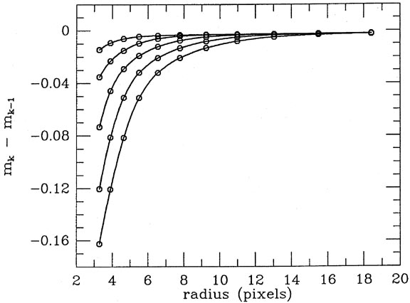
Figure 5-1.

Figure 5-2.
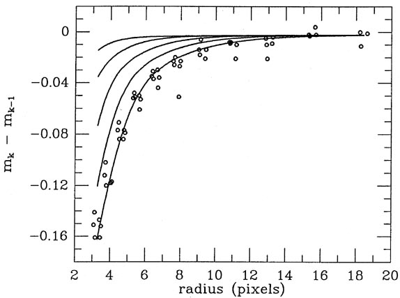
Figure 5-3.
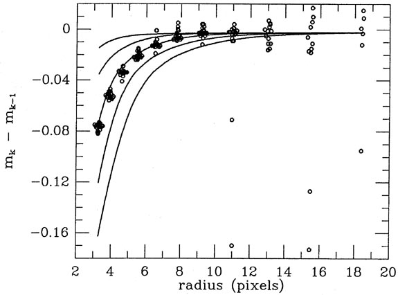
Figure 5-4.
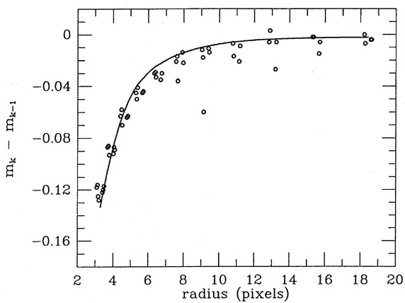
Figure 5-5.
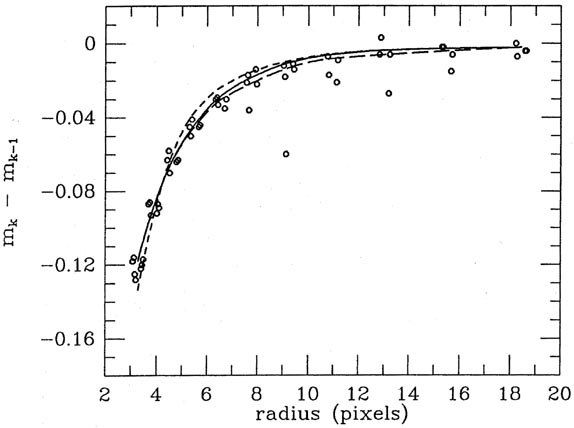
Figure 5-6.
 = 1. As I
discussed in the third lecture, this has
the effect of pulling the solution toward the median of the data points
(tinged toward the
mean of those data points with particularly small residuals). No datum
is so bad that it's
totally ignored. Even if the starting guesses are completely wrong,
still the solution will be
pulled into the center of the bulk of the data, rather than merely
latching onto whatever
lies closest to the starting guess. After the least-squares solution has
achieved a provisional
convergence with this clipping function, b is changed to 2
(a is left alone). This has the
effect of reducing the weights of the most discrepant points, while
slightly increasing the
weights of those points with small residuals (<
2
= 1. As I
discussed in the third lecture, this has
the effect of pulling the solution toward the median of the data points
(tinged toward the
mean of those data points with particularly small residuals). No datum
is so bad that it's
totally ignored. Even if the starting guesses are completely wrong,
still the solution will be
pulled into the center of the bulk of the data, rather than merely
latching onto whatever
lies closest to the starting guess. After the least-squares solution has
achieved a provisional
convergence with this clipping function, b is changed to 2
(a is left alone). This has the
effect of reducing the weights of the most discrepant points, while
slightly increasing the
weights of those points with small residuals (<
2 ); points with
moderate-to-large residuals
still carry some weight (a 4
residual still receives one-fifth weight, for instance. Look it
up: how often do you expect a
4 residual with a Gaussian error
distribution? Do you still
believe that cookbook least squares is the only truly honest way to
reduce data?). This
allows the solution to shift itself a little closer to where the data
points are thickest - it
adjusts itself more toward the mode of the raw data. Finally,
after this least-squares
solution has achieved provisional convergence, b is changed to 3. This
suppresses the really
bad observations still further, and restores the weights of the data
with small residuals to
a value still closer to unity. With this mechanism, I get most of the
best of both worlds:
I'm not stuck with including the obviously bad data points in my
results, and yet I don't
get paradoxical or non-unique answers. Regardless of the starting
guesses the solution is
pulled reliably and repeatably into the midst of the concordant
observations. By this time
I have looked at literally thousands of such solutions, and in every
case the final solution
has looked pretty much like what I would have sketched through the data
by hand and
eye, given the same information as the computer had.
Figs. 5-9 and 5-10
show the growth curves that were fitted to the data shown in
Figs. 5-7 and 5-8; for
comparison, I also show
the growth curves for two frames of similar seeing which contain
good raw data.
); points with
moderate-to-large residuals
still carry some weight (a 4
residual still receives one-fifth weight, for instance. Look it
up: how often do you expect a
4 residual with a Gaussian error
distribution? Do you still
believe that cookbook least squares is the only truly honest way to
reduce data?). This
allows the solution to shift itself a little closer to where the data
points are thickest - it
adjusts itself more toward the mode of the raw data. Finally,
after this least-squares
solution has achieved provisional convergence, b is changed to 3. This
suppresses the really
bad observations still further, and restores the weights of the data
with small residuals to
a value still closer to unity. With this mechanism, I get most of the
best of both worlds:
I'm not stuck with including the obviously bad data points in my
results, and yet I don't
get paradoxical or non-unique answers. Regardless of the starting
guesses the solution is
pulled reliably and repeatably into the midst of the concordant
observations. By this time
I have looked at literally thousands of such solutions, and in every
case the final solution
has looked pretty much like what I would have sketched through the data
by hand and
eye, given the same information as the computer had.
Figs. 5-9 and 5-10
show the growth curves that were fitted to the data shown in
Figs. 5-7 and 5-8; for
comparison, I also show
the growth curves for two frames of similar seeing which contain
good raw data.
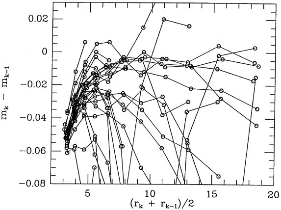
Figure 5-7.
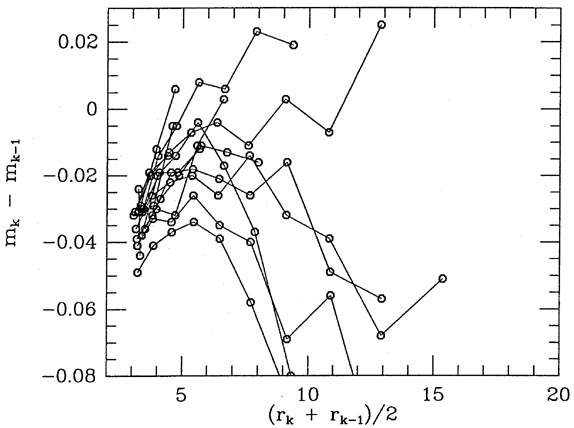
Figure 5-8.
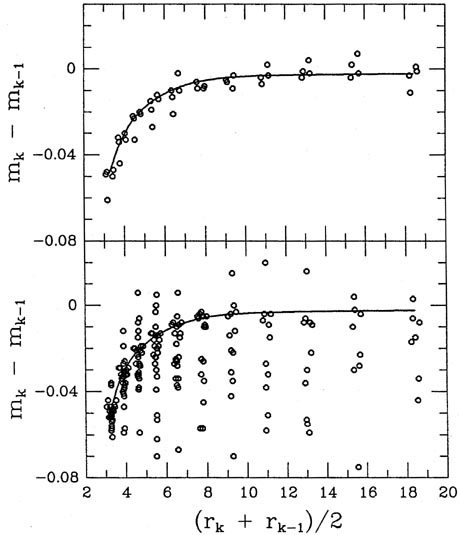
Figure 5-9.
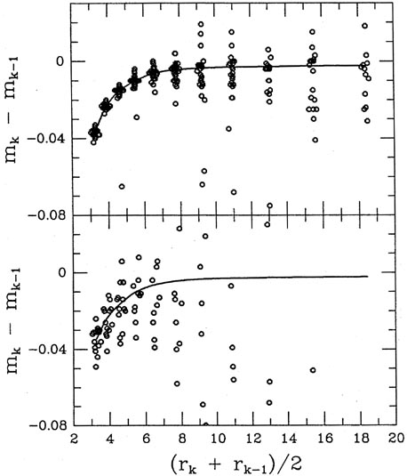
Figure 5-10.