2.1 The Fishing Trip

Take the last point first. Suppose that we have plotted something against something, on a ``fishing expedition'' of this type. There are grave dangers involved in this expedition, and we must ask ourselves the following questions.

1. Does the eye see much correlation? If not, calculation of a formal correlation statistic is probably a waste of time.

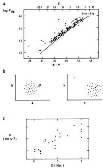
2. Could the apparent correlation be a result of selection effects? Consider, for instance, the beautiful correlation in Fig. 1(a), in which Sandage (1972) plotted radio luminosities of sources in the 3CR catalogue as a function of distance modulus. At first sight it proves luminosity evolution for radio sources. Are not the more distant objects (at earlier epochs) clearly the more powerful? In fact, as Sandage recognized, it proves nothing of the kind. The sample is flux- (or apparent-intensity) limited; the solid line shows the flux density limit of the 3CR catalogue. The lower right-hand region can never be populated; such objects are too faint to show above the limit of the 3CR catalogue. But what about the upper left-hand region? Provided that the luminosity function (the true space density in objects per Mpc³) slopes downward with increasing luminosity, the objects are bound to crowd towards the line. This is about all that can be gleaned immediately from the diagram - the space density of powerful radio sources is less than the space density of their weaker brethren. The diagram says nothing about the epoch dependence of properties of radio sources.

Fig. 1. Examples of ``correlations''. (a) The radio luminosity of identifications with radio sources in the 3CR catalogue versus distance modulus (Sandage 1972); dots are radio galaxies, crosses are quasars. The solid line shows the flux density limit of the 3CR catalogue. (b) Fictitious plots, for which formal test would indicate significant correlation but whose forms strongly suggest that data errors or selection effects would be responsible. (c) An early Hubble diagram (Hubble 1936), a plot of radial velocity versus distance to galaxies as estimated by their angular size.

It is worth emphasizing the lesson of the diagram. Astronomers produce many plots of this type, and will describe purported correlations in terms such as ``the lower right-hand region of the diagram is unpopulated because of the detection limit, but there is no reason why objects in the upper left-hand region should have escaped detection. . .''. True, but nor can they escape probability; the upper left of Sandage's diagram is not filled with QSOs and radio galaxies because in order to have a hope of encountering a powerful radio source we need to sample large spheres about us (3C273 is fortuitously close). Small spheres, corresponding to small redshifts and small distance moduli, will yield only low-luminosity radio sources because their space density is so much the higher. The lesson applies to any proposed correlation for variables with steep probability density functions dependent upon one of the variables plotted.

3. If we are happy about (2), we can try formal calculation of the significance of the correlation as described in Section 2.2. Further, if there is a correlation, does the regression line (Section 3.1) make sense?

4. If we are still happy, we must return to the plot to ask if the formal result is realistic. A rule of thumb - if 10 per cent of the points are grouped by themselves so that covering them with the thumb destroys the correlation to the eye, then we should doubt the result, no matter what significance level we have found. Beware, in particular, of plots that look like those of Fig. 1(b), plots which strongly suggest selection effects, data errors or some other form of statistical conspiracy.

5. If we are still confident, we must remember that a correlation does not prove a causal connection. The essential point is that correlation may simply indicate a dependence of both variables on a third variable. Cigarette manufacturers said so for years; but finding the physical attribute that caused heart/lung disease and the desire to smoke proved difficult. But there are many famous instances, e.g. the correlation between the general knowledge of children and their height, and between the size of feet in China and the price of fish in Billingsgate Market. For the former the hidden variable is age (Are tall children cleverer? No, but they are older), while for the latter it is time.

There are in fact ways of searching for intrinsic correlations between variables when they are known to depend mutually upon a third variable. The problem, however, when on the fishing trip, is how to know about a third variable, how to identify it when we might suspect that it is lurking. Partial correlation is a science in itself; it is covered in both parametric and non-parametric forms by Stuart & Ord (1991), Macklin (1982), and Siegel & Castellan (1988).

Finally we must not become too discouraged by all the foregoing. Consider Fig. 1(c), a ragged correlation if ever there was one, although there are no nasty groupings of the type rejected by the rule of thumb. It is in fact one of the earliest ``Hubble diagrams'' - the discovery of the recession of the nebulae, and the expanding Universe (Hubble 1936).