


3.3 Bayes Estimation
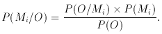
The ML principle is in contrast to what is sometimes known as Bayes's Postulate, which is the hypothesis that knowing nothing to the contrary, the a priori probabilities should all be taken as equal. Bayes' (3) Theorem enables computation of the a posteriori probabilities, and the choice of hypothesis is then made on the basis of the largest a posteriori probability. In general, this leads to answers different from ML; and other ``reasonable'' starting points yield different answers again.
It is the Postulate and not the Theorem that provides the continuing debate amongst statisticians. The theorem itself is a short exercise in logic, basically provable in a couple of lines. It says simply
This is a statement about conditional probabilities: in words - the
(conditional) probability of model Mi being true, given the
observation O, is proportional to the product of the probability
of O if Mi is true, and the a priori
probability of Mi. The latter term,
the ``priors'' in the jargon, contains the dynamite; Bayes' Postulate
would have that all of these are equal if we know nothing. However, we
always knew something at the start of our experiment; for instance,
intensities in an observed brightness distribution must be
positive. Thus on the one hand the Bayesian approach is very clever in
allowing us to incorporate prior information in a formal way; on the
other hand, just what form this information takes and how strongly one
should favour it in the light of the observation O is truly difficult
to assess.
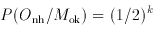
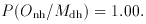
By way of contrived example, consider the proverbial bad penny, for
which prior information has indicated that there is a probability of
0.99 that it is unbiased (``ok''); or a probability of 0.01 that it is
double headed (``dh''). These then are the two models and their priors:
P (Mok) = 0.99; P
(Mdh) = 0.01. Let us toss the coin and use Bayes to
revise our view of the probability to be associated with the models.
Supposing we obtain n heads in a row, i.e. Onh
for the first n tosses.
Now
while
and
Plugging the numbers into Bayes's Theorem, for n = 2 we find
P (Onh / Mok) = 0.961; but by
n = 7 we find 0.436, i.e. less than a 50
percent chance that this coin is good. What decision would you make -
if forced to do so - on the basis of this evidence? On the one hand we
have cleverly made use of prior information in a formal way. On the
other hand, would we retain this information? Or what might our
judgement be of the experiment or person providing us with this
information? (For the most part even the strongest proponents of
Bayesian methods recognize that when the a posteriori results are
strongly sensitive to the priors, acquisition of more data should take
priority over debating the choice of these priors.)
By way of an astrophysical example, consider object detection for
which the prior is provided by the previously determined source count,
or N (S) number-flux-density law. The Bayesian best estimate of
detected intensity must be modified by the known N (S) relation, and it
happens that this modification is the same as that for the
maximum-likelihood estimate
(Jauncey 1968).
If carried to strict
formality, every time a detection is made all other catalogued flux
densities should be modified. Moreover, in the extragalactic radio
source situation, the source count is actually different for different
types of optical counterpart, e.g. radio galaxy or QSO. Does this mean
that the nature of the subsequent optical identification after radio
detection changes the radio flux density? Could we in fact identify an
object, ``change'' its flux density, and find that it is then below the
a priori radio detection limit?
The answer must be that there are types of modelling and
experimentation to which Bayesian methods lend themselves readily;
there are other types of experiment for which the application will do
little toward decision making but much towards controversy.
A fundamental work of reference on Bayesian methods is that by
Jeffreys (1961);
the antidote, the frequentist viewpoint, is from
Edwards (1972).
An excellent overview is provided by
Jaynes (1986),
and some modern treatments (e.g.
Bernardo & Smith 1994,
Berry 1996)
are also highly readable and provide balanced views of Bayesian versus
frequentist approaches. The former provides a comprehensive reference
list, while the latter has a particularly simple approach with many
worked examples. One of the most interesting uses of such methods for
modelling in astronomy is the maximum-entropy technique for mapping
developed by Gull and collaborators
(Gull & Daniel 1978;
Gull & Skilling 1984).
A popular and less controversial technique for model fitting based
on an entirely different premise is given in the following section.

3 Who was Bayes? Thomas Bayes (1702-61),
English vicar, mathematician,
statistician - his bibliography consisted of three works: one (by the
vicar) on Divine Providence, the second (by the mathematician) a
defence of the logical bases of Newton's calculus against the attacks
of Bishop Berkeley, and the third (by the statistician and published
posthumously) the famous Essay towards solving a problem in the
doctrine of chances
(Bayes 1763).
There is speculation that it was
published posthumously because of the controversy that Bayes believed
would ensue. This must be an a posteriori judgement. Surely Bayes
could never have imagined the extent of this controversy without
envisaging the nature and extent of modern scientific data.
Back.