C. The Friedmann Models
To describe the expansion of the universe one must use the RWM along with the Einstein equations,
to determine the equations of motion. For reference, a summary of
the metric coefficients, the Christoffel Symbols, and the Ricci
Tensor components are presented in
[13, Chapter 15].
Note that in this book the scale factor a(t) is written R(t).
Before proceeding any further, an appropriate stress-energy tensor
must be provided. This is the difficult part of the process. The
composition of the known universe is a very controversial topic.
The standard procedure is to consider simplified distributions of
mass and energy to get an approximate model for how the universe
evolves.
At this point, units are chosen such that the speed of light, c
is set equal to unity. This gives the simplification that the
energy density,
where p is the pressure,
At the earliest epoch of the universe, the contribution of photons
to the energy density would have been appreciable. However, as the
universe cooled below a critical temperature, allowing the photons
to decouple from baryonic matter, the photon contribution became
negligible. Thus, it is easier to consider different energy
distributions for different epochs in the universe. The massive
contribution to the energy density is usually referred to as the
Baryonic contribution, since baryons (protons, neutrons, etc.) are
significantly more massive than leptons (electrons, positrons,
etc.) and leptons can therefore be disregarded as a major
contributing factor to the total energy density. There is also the
contribution of vacuum energy, which enters the Einstein equations
through the cosmological constant,
For each type of contribution, there is a corresponding density,
Furthermore, assuming that one is dealing with a
homogeneous and isotropic fluid, the density can be related to the
pressure by a simple equation of state (see Table 1),
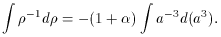
Another useful relation involves the Conservation of Energy
(1st Law of Thermodynamics). Assuming the ideal fluid expands
adiabatically, one finds
[14],
which may be rewritten as,
Relating (11) and (12) gives,
Using the product rule,
Which can be integrated,
In the Radiation epoch, where the energy density due to photons
was appreciable (from about t = 0 to approximately 300,000 years
after the Big-Bang
[15]), the
density due to massive
particles can be neglected. The pressure is found to be equal to
a third of the density, and we have a value of one-third for
Following this epoch, the Matter Dominated epoch can be modeled
after a `dust' that uniformly fills space. Because the temperature
of the universe had fallen to around 3000 K, most of the particles
had non-relativistic velocities (v << c). This corresponds to a
negligible pressure and
The last case to consider is that of the vacuum energy. If the
cosmological constant is indeed nonzero, this form of energy
density will dominate. For this relation, the pressure is
commensurate with that of a negative density. This would imply a
value of -1 for
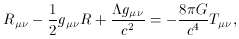
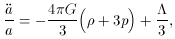
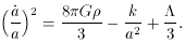
Given an expression for the energy-momentum tensor, one can now
proceed to find the equations of motion. The metric coefficients
follow from the Robertson Walker line element, which is given by
equation (4). Using these coefficients one can
obtain the expression for the left side of the Einstein equations
(8). Thus, from the Einstein equations one
derives the Friedmann equations in their most general form:
Apparently, if the universe is in a vacuum dominated state
p = -
Now is the time to introduce a bit of machinery to make our
calculations more tractable. Recall that the Hubble constant,
H(t), is defined as
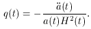
Next, one defines the Deceleration parameter (named for historical
reasons) as,
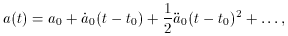
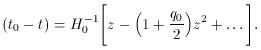
To realize how this term arises, consider the Taylor
expansion of the scale factor, about the present time, t0,
where the sub-zeros indicate the terms are evaluated at the
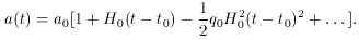
present. Using equations (16) and (17), this
becomes
Remembering that the crux for obtaining Hubble's Law (1) was measuring
the luminosity distance, it is of interest to
consider this calculation quantitatively. The flux F (energy
per time per area received by the detector) is defined in terms of
the known luminosity L (energy per time emitted in the star's
rest frame) and the luminosity distance dL.
The luminosity distance must take into account the
expanding universe and can be written in terms of the redshift,
z as [5],
where a0 is the present scale factor and r is
the comoving
coordinate that parameterizes the space. Hubble used the measured
flux and the known luminosity to find the distance to the objects
he measured. The distance can then be compared with the known
redshift of the object using (20) and the velocity can
be approximated. However, r in (20) is not a
observable and it is of interest to examine the great amount of
estimation that must be used to derive the desired result
analytically.
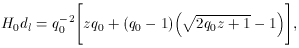
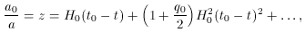
Dividing (18) by a0 and making use of (7) yields,
which can be solved for (t0 - t),
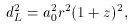
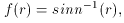
One can also expand (6) in a power series,
where re has been replaced by r (for
simplicity) and sin n-1 (r) is defined as
sin1 (r) for
k = 1, sinh-1 (r) for k = -1 and
r for k = 0. So to lowest
order, (6) can be estimated as r, and the l.h.s.
of (6) can be estimated as,
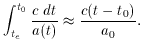
Using the approximation from (23) and the
above result we have,
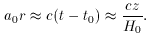
Substitution of t - t0 from (22) and keeping
only lowest order terms yields,
At small redshift, z << 1 one finds z
where dp is the physical distance. Thus, we have obtained
Hubble's law (1) as an approximation. This
derivation reflects the reason that the law only holds locally.
The number of approximations that were needed to proceed was
appreciable. Furthermore, one finds that this law deviates
significantly at large z as one would expect.
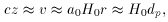
For a matter dominated model, one finds the exact Hubble relation
to be given by [5],
which depends on the deceleration parameter,
q0, which in turn relies on the curvature and the total mass
density of the universe.
 is equal
to the mass density,
is equal
to the mass density,  using, =
c2 =
. This also allows mass and
energy to be considered together, which is in the spirit of the
stress-energy tensor. The mass/energy density will be referred to
as the energy density for the remainder of this paper. The
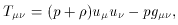
stress-energy tensor may be given as:
using, =
c2 =
. This also allows mass and
energy to be considered together, which is in the spirit of the
stress-energy tensor. The mass/energy density will be referred to
as the energy density for the remainder of this paper. The
stress-energy tensor may be given as:
 is the density, and
uµ is the four-velocity.
is the density, and
uµ is the four-velocity.
 .
. The total density
can be expressed as the sum of the different contributions as
.
. The total density
can be expressed as the sum of the different contributions as

Density
Pressure p

Epoch
R
/3
1/3
Radiation Dominated
M
0
0
Matter Dominated (Non-relativistic Dust)
-
-1
Vacuum Domination

 , so
R ~
a-4
[9].
is
therefore zero,
~ constant
[9].
, so
M ~
a-3
[9].
These results are summarized in Table 1.
, so
R ~
a-4
[9].
is
therefore zero,
~ constant
[9].
, so
M ~
a-3
[9].
These results are summarized in Table 1.
 , (14)
indicates the universe will be accelerating.
This important conclusion will be the most general requirement for
an inflationary model.
, (14)
indicates the universe will be accelerating.
This important conclusion will be the most general requirement for
an inflationary model.


 v/c. Thus, making
this final approximation one obtains,
v/c. Thus, making
this final approximation one obtains,