B. Inflation As a Solution to the Initial Value Problems

It was discussed in the first part of this section that inflation solves the flatness problem because the universe expands at such a great rate that the curvature term is `redshifted' away. Another way of stating this result is to define inflation as any period in the evolution of the universe in which the scale factor (a(t)) undergoes a period of acceleration; i.e., (t) > 0. This condition can be used to provide a further insight into what inflation means. Consider the quantity (H a)^-2. Knowing

it follows that

Now consider the time derivative of this quantity.

given the conditions > 0 and > 0. This implies,

(48)

Referring back to equation (45), and dividing through by H², one again gets the equation for the evolution of the density parameter, = / _c,

(49)

Comparing Equations (48) and (49) expresses the fact that the curvature decreases during inflation. More explicitly, as a and H increase by tremendous amounts during inflation, the right had side of (49) approaches zero since the denominator becomes large. Thus, is driven towards one and the universe is made flat by inflation. As the scale factor evolves under the condition > 0 the density () approaches the critical density (_c).

But (48) can also be written as, d(1/Ha)/dt < 0 since H and a are both taken as positive quanitites. Recall that 1/H gives the particle horizon of a flat universe, so one can use Equation (5),

where r is the comoving radial coordinate. Using d(1/Ha)/dt < 0 gives the relation,

What does this mean? This implies that during a period of inflation the comoving frame (parameterized by r, , and ), SHRINKS! Remember that the comoving coordinates represent the system of coordinates that are at rest with respect to the expansion. In other words, instead of viewing the spacetime as expanding it is equally valid to view the particle horizon as shrinking. To visualize this, it is perhaps useful to again consider the idea of an expanding balloon (see Figures 3 and 4). Normally, in this example, one views two points on the surface of the balloon as getting farther apart because the balloon is expanding. However, if one chooses a frame in which the surface is not expanding this would mean that the metric, or way of measuring, would shrink. Thus, the distance between the points would get larger, since the comoving coordinates got smaller. Each frame of reference has its advantages. For the remainder of this paper I will choose the frame where the universe is seen to expand. This has the advantage that the Hubble length remains `almost' constant during inflation, which eases the discussion in the analysis to follow.

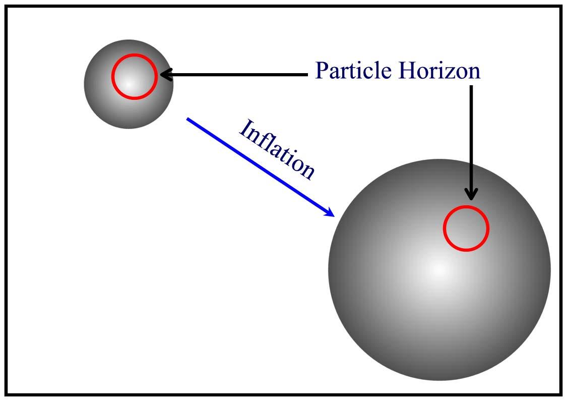
Figure 3. This figure illustrates the expansion from the point of view of an observer located in an embedded dimension. In this way, the observer can `look down' and see the expansion take place. The spacetime is seen to expand from under the particle horizon.

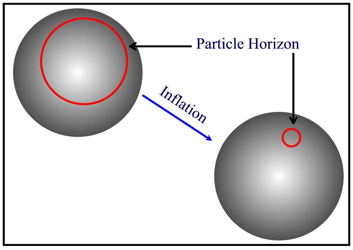
Figure 4. This figure illustrates the more natural perspective contrasted to that of Figure (3). The frame of reference is that of comoving coordinates, which puts the observer at rest relative to the expansion. In this frame the particle horizon is seen to shrink.

So, the picture during inflation is that the spacetime background expands at an accelerating pace. This resolves the horizon problem, since causal regions in the early universe are stretched to regions much larger than the Hubble distance. This is because during inflation the scale factor evolves at super-luminal speeds, whereas the particle horizon (Hubble distance) is approximately constant. The particle horizon does expand at the speed of light (by definition), but this pales in comparison to the evolution of the scale factor. Remember the Hubble distance is the farthest distance light could have traveled from a source to reach an observer. Once inflation ends, the scale factor returns to its sub-luminal evolution leaving the particle horizon to ``catch up''. This situation is illustrated in Figure 5. So as we look out at the sky today we are still seeing the regions of uniformity that were stretched outside the particle horizon during inflation.

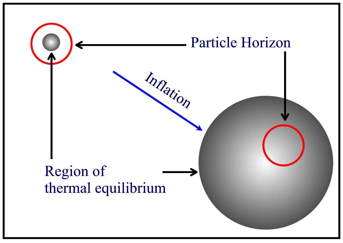
Figure 5. This figure illustrates that during inflation regions that have achieved thermal equilibrium can be expanded outside the particle horizon (Hubble distance). After inflation, the particle horizon begins to expand faster than the spacetime and these regions reenter the horizon. Inflation is the only known way to explain this uniformity, thus solving the horizon problem.

With the discussion presented thus far, the monopole problem is solved trivially. The number of predicted monopoles per particle horizon at the onset of inflation is on the order of one [42]. As discussed previously, this would result in a density today that would force >> 1, which is not observed. As stated previously, the comoving (causal) horizon shrinks during inflation. Thus, if the universe starts with one monopole, it may contain that one monopole after inflation, but no more. However, this is highly unlikely if the universe inflates by an appreciative amount. Furthermore, inflation redshifts all energy densities. So, as long as the temperature does not go near the critical temperature after inflation, no additional monopoles may form.

This holds true for the other topological defects and unwanted relics associated with spontaneous symmetry breaking (SSB) in unified theories. This leads one to ask, why would the temperature increase after inflation? The mechanism by which this reheating of the universe takes place is related to the mechanisms that bring about the demise of the inflationary period. These mechanisms are understood through the dynamics of scalar fields, to be discussed in the next section.

One question has been left unresolved with reference to the problems of initial values in the hot Big Bang model. This is the problem of the origin of structure in the universe. It was pointed out that the DeSitter universe is left empty and cold with no stars or galaxies. The flatness and monopole problem were resolved by a redshifting of the various energy densities. But, if no energy is present, how can particle creation take place? This peculiar feature of inflation will be discussed in the next section, but here I would like to present a qualitative description.

At the end of inflation, all energy densities have become negligible except the vacuum density (or cosmological constant if you prefer). Where did the energy go? It went into the gravitational `potential' of the universe, so energy is still conserved [43], [44] <sup>(24)</sup> Thus, at the end of inflation there is a universe filled with vacuum energy, which takes the form of a scalar field. This scalar field is coupled to gauge fields, such as the photon. As the scalar field releases its energy to the coupled field, the universe goes through a reheating phase where particles are created as in the hot Big Bang model. The energy for this particle creation is provided by the `latent' heat locked in the scalar field. More will be said on this later, but the important point is that the hot Big Bang model picks up where inflation leaves off. Thus, one may be inclined to say, inflation is a slight modification to the hot Big Bang model. One author refers to inflation as, ``a bolt on accessory'' [29].

This all sounds very appealing, however reheating is a fragile topic for inflation and results in a number of different models. This derives from the fact that if the temperature is too high at the time of reheating, the unwanted particle relics could be re-introduced into the model! As a result, many different reheating scenarios have been proposed, along with many different models for the onset of inflation.

One surprise from inflation makes all of this worry worth it. Along with offering a solution to the various initial value problems of the hot Big Bang, inflation offers a mechanism to seed the large-scale structure of the universe. Depending on the model chosen, (e.g., reheating temperature, onset conditions, etc.) one gets predictions for the large-scale structure of the universe and the anisotropies in the cosmic background. As will be seen in the next section, this again demonstrates how the very small (quantum mechanics) can impact the very large (universal structure). In some models of inflation, a small fluctuation in the quantum foam of the Planck epoch (t < 10^-43) can give rise to the formation of galaxies, solar systems, and eventually human life! We are the result of pure chance! This is getting a little ahead of the game, so let us consider a quantitative and mechanical explanation of inflation.

²⁴ Actually, energy need not be conserved if we live in an open universe. However, this need not concern us here. Back.