Distance scale and peculiar velocity work have long been plagued by statistical biases. These biases are sufficiently confusing and multifaceted that their effects are often misunderstood or misrepresented. It is worth taking a moment to go over a few of the main issues.
The root problem is that our distance indicators contain
scatter: a galaxy with distance d inferred from the DI
really lies within some range of distances, approximately
(but not exactly) centered on d. This range is characterized
by a non-gaussian distribution of characteristic width d , where
is the fractional distance
error characteristic
of the DI. (If
, where
is the fractional distance
error characteristic
of the DI. (If  is the DI
scatter in magnitudes,
is the DI
scatter in magnitudes,
 0.46 ). Thus,
the farther away the object is the bigger the distance error.
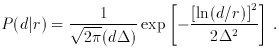
For most DIs, a good approximation is that
the distribution of distance errors is
log-normal: if the true distance is r,
then the distance estimate d has a probability distribution
given by
0.46 ). Thus,
the farther away the object is the bigger the distance error.
For most DIs, a good approximation is that
the distribution of distance errors is
log-normal: if the true distance is r,
then the distance estimate d has a probability distribution
given by
Two distinct kinds of statistical bias effects can arise when
DIs with the above properties are used.
Which of the two occurs depends on which of two
basic analytic approaches one adopts for treating
the DI data. In the first approach, known as Method I,
one assumes that the DI-inferred distance d is the
best a priori estimate of true distance. Any subsequent
averaging or modeling of the data points assumes galaxies
with similar values of d to be neighbors in real space
as well. The second approach, known as Method II,
takes proximity in redshift space as tantamount to
real-space proximity; the DI-inferred distances
are then treated only in a statistical sense, averaged
over objects with similar redshift-space positions.
The Method I/Method II terminology
originated with
Faber & Burstein
(1988);
a detailed discussion is provided by
Strauss & Willick (1995,
Section 6.4).
Let us consider this distinction in relation
to peculiar velocity or Hubble constant studies.
In a Method I approach, one would take
objects whose DI-inferred
distances are within a narrow range of some value d,
and average their redshifts. Subtracting
d from the resulting mean redshift yields a peculiar velocity estimate;
dividing the mean redshift by d gives an estimate of
H0.
However, these estimates will be biased, because the distance
estimate d itself is biased:
It is not the mean true distance of the objects in question.
To see this, we reason as follows: if P (d|r) is given
by equation 12 above, then the distribution of
true distances of our objects is given, according to Bayes' Theorem, by
where we have taken P(r)
The biases which arise in a Method II analysis are quite different.
They may be rigorously understood in terms of the probability distribution
of the DI-inferred distance d given the redshift cz,
P (d|cz) (contrast with equation 13, which
underlies Method I). In general, this distribution
is quite complicated (cf.
Strauss & Willick
1995,
Section 8.1.2),
and its details are beyond the scope of this Chapter.
However, under the assumption of a ``cold'' velocity field - an
assumption that appears adequate in ordinary environments - redshifts
complemented by a flow model
give a good approximation of true distance. Thus, it really is the
probability distribution P (d|r) (equation (12), or
one similar to it,
that counts for a Method II analysis. However, that equation as written
does not represent the full story. If severe
selection effects such as a magnitude or diameter limit
are present, then the log-normal distribution does not apply exactly.
Some galaxies are too faint or small to be in the
sample; in effect, the large-distance tail of P(d|r)
is cut off. It follows that
the typical inferred distances are smaller than
those expected at a given true distance r.
As a result, the peculiar velocity model that
allows true distance to be estimated as a function of redshift is
tricked into returning shorter distances. This bias goes
in the same sense as Malmquist bias, but is fundamentally
different. It results not from volume/density effects,
but from sample selection effects, and
is called selection bias.
Selection bias can be avoided, or at least minimized, by
working in the so-called ``inverse direction.'' What that
means is most easily illustrated using the
TF relation. When viewed in its ``forward'' sense,
the TF relation is conceived as a prediction of
absolute magnitude given a value of the velocity
width parameter, M(
This fact, first clearly stated by
Schechter (1980) and
then reiterated in various forms by
Aaronson et
al. (1982),
Tully (1988),
Willick (1994),
Dekel (1994), and
Davis et al. (1996),
among others, remains an obscure one, not universally
appreciated. It is often heard, for example, that the TF
relation applied to relatively distant galaxies will necessarily
result in a Hubble constant that is biased high, because
the distances are biased low due to selection bias.
The clear conclusion of the previous paragraph, however, is that provided the
analysis is done using redshift-space information to assign a priori
distances - that is, provided that a Method II
approach is taken - working in the inverse direction can render selection
bias unimportant. It is also the case that a careful analytical methods
(Willick 1994)
can permit a correction for selection
bias even when working in the forward direction. It should
be borne in mind, however, that both of these approaches
(using the inverse relation or correction for forward selection
bias) necessitate a careful characterization of sample
selection criteria.
Another wrinkle in this complicated subject is that the
relatively bias-free character of inverse distance indicators
does not carry over to a Method I analysis. It is beyond the
scope of this Chapter to discuss this issue in full detail;
the interested reader is referred to Strauss & Willick
(1995,
Section 6.5). The main point is that a Method I inverse DI analysis
is subject to Malmquist bias in much the same way as a
Method I forward analysis; indeed, the inverse Malmquist
bias is in some ways considerably more complex, as it
depends (unlike forward Malmquist bias)
on sample selection criteria. So while it is correct
to emphasize the bias-free (or nearly so) nature of
working in the inverse direction, it is essential
to remember that this property holds only for Method
II analyses.
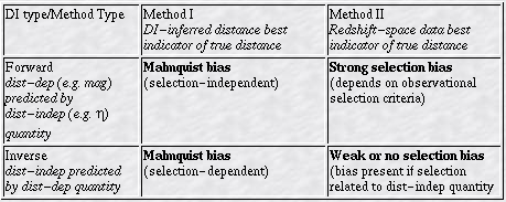
Much of the confusion surrounding the
relative bias properties of forward versus inverse
DIs stems from neglecting the distinction between
Method I and Method II analyses. Recognizing this,
Strauss & Willick
(1995)
summarized the issue with what they called the ``Method Matrix''
(a more memorable term might be the ``magic square'')
of peculiar velocity analysis.
Their table is reproduced above, in a slightly simpler
form (the original alluded to several complications
that are unecessary here).
Reference to this simple diagram might allay some of the
controversies surrounding Malmquist and related biases.
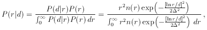
 r2 n(r), where n(r) is the
underlying galaxy number density along the line of sight.
To obtain the expectation value of the
true distance r for a given d, we
multiply equation (13)
by r and integrate over all r. In general, this
integral requires knowledge of the density field n(r)
and will have to be done numerically. However, in the
simplest case that the density field is constant, the
integral can be done analytically. The result is
that the expected true distance is de72/2
(Lynden-Bell et
al. 1988;
Willick 1991).
This effect is called homogeneous Malmquist bias. It tells
us that, typically, objects lie further away than their
DI-inferred distances. The physical cause
is more objects ``scatter in''
from larger true distances (where there is more volume)
than ``scatter out'' from smaller ones. In general, however, variations
in the number density cannot be neglected. When this is
the case, there is inhomogeneous Malmquist bias (IHM).
IHM can be computed numerically if one has a model of
the density field. Further discussion of this issue
may be found in
Willick et al. (1997).
r2 n(r), where n(r) is the
underlying galaxy number density along the line of sight.
To obtain the expectation value of the
true distance r for a given d, we
multiply equation (13)
by r and integrate over all r. In general, this
integral requires knowledge of the density field n(r)
and will have to be done numerically. However, in the
simplest case that the density field is constant, the
integral can be done analytically. The result is
that the expected true distance is de72/2
(Lynden-Bell et
al. 1988;
Willick 1991).
This effect is called homogeneous Malmquist bias. It tells
us that, typically, objects lie further away than their
DI-inferred distances. The physical cause
is more objects ``scatter in''
from larger true distances (where there is more volume)
than ``scatter out'' from smaller ones. In general, however, variations
in the number density cannot be neglected. When this is
the case, there is inhomogeneous Malmquist bias (IHM).
IHM can be computed numerically if one has a model of
the density field. Further discussion of this issue
may be found in
Willick et al. (1997).
 ). However, it is equally
valid to view the relation as a prediction of
given a value of M, i.e., as a function 0 (M)
(the superscript ensures that there is no confusion
between the observed width parameter and the
TF-prediction). When one uses the forward relation,
one imagines fitting a line mi = M (i) +
µ by regressing
the apparent magnitudes mi on the velocity widths i;
the distance modulus µ
is the free parameter solved for. Selection bias then
occurs because apparent magnitudes fainter than
the magnitude limit are ``missing'' from the
sample, so the fitted line is not the same
as the true line. However, if one instead fits a line
0
(mi - µ) by regressing the widths on the
magnitudes, the same effect does not occur, provided
the sample selection procedure does not exclude large
or small velocity widths. In general, this last caveat
is more or less valid. Consequently, working in the
inverse direction does in fact avoid or at least minimize
selection bias.
). However, it is equally
valid to view the relation as a prediction of
given a value of M, i.e., as a function 0 (M)
(the superscript ensures that there is no confusion
between the observed width parameter and the
TF-prediction). When one uses the forward relation,
one imagines fitting a line mi = M (i) +
µ by regressing
the apparent magnitudes mi on the velocity widths i;
the distance modulus µ
is the free parameter solved for. Selection bias then
occurs because apparent magnitudes fainter than
the magnitude limit are ``missing'' from the
sample, so the fitted line is not the same
as the true line. However, if one instead fits a line
0
(mi - µ) by regressing the widths on the
magnitudes, the same effect does not occur, provided
the sample selection procedure does not exclude large
or small velocity widths. In general, this last caveat
is more or less valid. Consequently, working in the
inverse direction does in fact avoid or at least minimize
selection bias.